4.3: Inferences about Two Means with Dependent Samples—Matched Pairs
- Page ID
- 2892
\( \newcommand{\vecs}[1]{\overset { \scriptstyle \rightharpoonup} {\mathbf{#1}} } \)
\( \newcommand{\vecd}[1]{\overset{-\!-\!\rightharpoonup}{\vphantom{a}\smash {#1}}} \)
\( \newcommand{\id}{\mathrm{id}}\) \( \newcommand{\Span}{\mathrm{span}}\)
( \newcommand{\kernel}{\mathrm{null}\,}\) \( \newcommand{\range}{\mathrm{range}\,}\)
\( \newcommand{\RealPart}{\mathrm{Re}}\) \( \newcommand{\ImaginaryPart}{\mathrm{Im}}\)
\( \newcommand{\Argument}{\mathrm{Arg}}\) \( \newcommand{\norm}[1]{\| #1 \|}\)
\( \newcommand{\inner}[2]{\langle #1, #2 \rangle}\)
\( \newcommand{\Span}{\mathrm{span}}\)
\( \newcommand{\id}{\mathrm{id}}\)
\( \newcommand{\Span}{\mathrm{span}}\)
\( \newcommand{\kernel}{\mathrm{null}\,}\)
\( \newcommand{\range}{\mathrm{range}\,}\)
\( \newcommand{\RealPart}{\mathrm{Re}}\)
\( \newcommand{\ImaginaryPart}{\mathrm{Im}}\)
\( \newcommand{\Argument}{\mathrm{Arg}}\)
\( \newcommand{\norm}[1]{\| #1 \|}\)
\( \newcommand{\inner}[2]{\langle #1, #2 \rangle}\)
\( \newcommand{\Span}{\mathrm{span}}\) \( \newcommand{\AA}{\unicode[.8,0]{x212B}}\)
\( \newcommand{\vectorA}[1]{\vec{#1}} % arrow\)
\( \newcommand{\vectorAt}[1]{\vec{\text{#1}}} % arrow\)
\( \newcommand{\vectorB}[1]{\overset { \scriptstyle \rightharpoonup} {\mathbf{#1}} } \)
\( \newcommand{\vectorC}[1]{\textbf{#1}} \)
\( \newcommand{\vectorD}[1]{\overrightarrow{#1}} \)
\( \newcommand{\vectorDt}[1]{\overrightarrow{\text{#1}}} \)
\( \newcommand{\vectE}[1]{\overset{-\!-\!\rightharpoonup}{\vphantom{a}\smash{\mathbf {#1}}}} \)
\( \newcommand{\vecs}[1]{\overset { \scriptstyle \rightharpoonup} {\mathbf{#1}} } \)
\( \newcommand{\vecd}[1]{\overset{-\!-\!\rightharpoonup}{\vphantom{a}\smash {#1}}} \)
\(\newcommand{\avec}{\mathbf a}\) \(\newcommand{\bvec}{\mathbf b}\) \(\newcommand{\cvec}{\mathbf c}\) \(\newcommand{\dvec}{\mathbf d}\) \(\newcommand{\dtil}{\widetilde{\mathbf d}}\) \(\newcommand{\evec}{\mathbf e}\) \(\newcommand{\fvec}{\mathbf f}\) \(\newcommand{\nvec}{\mathbf n}\) \(\newcommand{\pvec}{\mathbf p}\) \(\newcommand{\qvec}{\mathbf q}\) \(\newcommand{\svec}{\mathbf s}\) \(\newcommand{\tvec}{\mathbf t}\) \(\newcommand{\uvec}{\mathbf u}\) \(\newcommand{\vvec}{\mathbf v}\) \(\newcommand{\wvec}{\mathbf w}\) \(\newcommand{\xvec}{\mathbf x}\) \(\newcommand{\yvec}{\mathbf y}\) \(\newcommand{\zvec}{\mathbf z}\) \(\newcommand{\rvec}{\mathbf r}\) \(\newcommand{\mvec}{\mathbf m}\) \(\newcommand{\zerovec}{\mathbf 0}\) \(\newcommand{\onevec}{\mathbf 1}\) \(\newcommand{\real}{\mathbb R}\) \(\newcommand{\twovec}[2]{\left[\begin{array}{r}#1 \\ #2 \end{array}\right]}\) \(\newcommand{\ctwovec}[2]{\left[\begin{array}{c}#1 \\ #2 \end{array}\right]}\) \(\newcommand{\threevec}[3]{\left[\begin{array}{r}#1 \\ #2 \\ #3 \end{array}\right]}\) \(\newcommand{\cthreevec}[3]{\left[\begin{array}{c}#1 \\ #2 \\ #3 \end{array}\right]}\) \(\newcommand{\fourvec}[4]{\left[\begin{array}{r}#1 \\ #2 \\ #3 \\ #4 \end{array}\right]}\) \(\newcommand{\cfourvec}[4]{\left[\begin{array}{c}#1 \\ #2 \\ #3 \\ #4 \end{array}\right]}\) \(\newcommand{\fivevec}[5]{\left[\begin{array}{r}#1 \\ #2 \\ #3 \\ #4 \\ #5 \\ \end{array}\right]}\) \(\newcommand{\cfivevec}[5]{\left[\begin{array}{c}#1 \\ #2 \\ #3 \\ #4 \\ #5 \\ \end{array}\right]}\) \(\newcommand{\mattwo}[4]{\left[\begin{array}{rr}#1 \amp #2 \\ #3 \amp #4 \\ \end{array}\right]}\) \(\newcommand{\laspan}[1]{\text{Span}\{#1\}}\) \(\newcommand{\bcal}{\cal B}\) \(\newcommand{\ccal}{\cal C}\) \(\newcommand{\scal}{\cal S}\) \(\newcommand{\wcal}{\cal W}\) \(\newcommand{\ecal}{\cal E}\) \(\newcommand{\coords}[2]{\left\{#1\right\}_{#2}}\) \(\newcommand{\gray}[1]{\color{gray}{#1}}\) \(\newcommand{\lgray}[1]{\color{lightgray}{#1}}\) \(\newcommand{\rank}{\operatorname{rank}}\) \(\newcommand{\row}{\text{Row}}\) \(\newcommand{\col}{\text{Col}}\) \(\renewcommand{\row}{\text{Row}}\) \(\newcommand{\nul}{\text{Nul}}\) \(\newcommand{\var}{\text{Var}}\) \(\newcommand{\corr}{\text{corr}}\) \(\newcommand{\len}[1]{\left|#1\right|}\) \(\newcommand{\bbar}{\overline{\bvec}}\) \(\newcommand{\bhat}{\widehat{\bvec}}\) \(\newcommand{\bperp}{\bvec^\perp}\) \(\newcommand{\xhat}{\widehat{\xvec}}\) \(\newcommand{\vhat}{\widehat{\vvec}}\) \(\newcommand{\uhat}{\widehat{\uvec}}\) \(\newcommand{\what}{\widehat{\wvec}}\) \(\newcommand{\Sighat}{\widehat{\Sigma}}\) \(\newcommand{\lt}{<}\) \(\newcommand{\gt}{>}\) \(\newcommand{\amp}{&}\) \(\definecolor{fillinmathshade}{gray}{0.9}\)Inferences about Two Means with Dependent Samples—Matched Pairs
Dependent samples occur when there is a relationship between the samples. The data consists of matched pairs from random samples. A sampling method is dependent when the values selected for one sample are used to determine the values in the second sample. Before and after measurements on a population, such as people, lakes, or animals are an example of dependent samples. The objects in your sample are measured twice; measurements are taken at a certain point in time, and then re-taken at a later date. Dependency also occurs when the objects are related, such as eyes or tires on a car. Pairing isn’t a problem; it’s an opportunity to use the information that occurs with both measurements.
Before you begin your work, you must decide if your samples are dependent. If they are, you can take advantage of this fact. You can use this matching to better answer your research questions. Pairing data reduces measurement variability, which increases the accuracy of our statistical conclusions.
We use the difference (the subtraction) of the pairs of data in our analysis. For each pair, we subtract the values:
- \(d_1\) = before1 – after 1
- \(d_2\) = before 2 – after 2
- \(d_3\) = before 3 – after 3
- …
We are creating a new random variable d (differences), and it is important to keep the sign, whether positive or negative. We can compute d̄, the sample mean of the differences, and sd, the sample standard deviation of the differences as follows:
\[\bar {d} = \frac {\sum d_i}{n}\]
\[s_d = \sqrt {\frac {\sum (d-\bar{d})^2}{n-1}}\]
Just as we used the sample mean and the sample standard deviation in a one-sample t-test, we will use the sample mean and sample standard deviation of the differences to test for matched pairs. The assumption of normality must still be verified. The differences must be normally distributed or the sample size must be large enough (n ≥ 30).
We can do a hypothesis test using matched pairs data following the same methods we used in the previous chapter.
- Write the null and alternative hypotheses.
- State the level of significance and find the critical value.
- Compute a test statistic.
- Compare the test statistic to the critical value and state a conclusion.
Since we are using the differences between the pairs of data, we identify this in our null and alternative hypotheses: \(H_0: \mu d = 0\). The mean of the differences is equal to zero; there is no difference in “before and after” values.
We’ll use the same three pairs of null and alternative hypotheses we used in the previous chapter.
Table \(\PageIndex{1}\). Null and alternative hypotheses.
| Two-sided | Left-sided | Right=sided |
| \(\mathrm{H}_{\mathrm{0}}: \mu_d=c\) | \(\mathrm{H}_{\mathrm{0}}: \mu_d=\c \) | (\mathrm{H}_{\mathrm{0}}: \mu_d=c \) |
| \(\mathrm{H}_1: \mu_d \neq c\) | \(\mathrm{H}_1: \mu_d<c \) | \(\mathrm{H}_1: \mu_d>c \) |
Table 3. Null and alternative hypotheses.
The critical value comes from the student’s t-distribution table with n – 1 degrees of freedom, where n = number of matched pairs. The test statistic follows the student’s t-distribution
\[t=\frac {\bar {d}-\mu_d}{(s_d/\sqrt {n})}\]
The conclusion must always answer the question you are asking in the alternative hypothesis.
- Reject the \(H_0\). There is enough evidence to support the alternative claim.
- Fail to reject the \(H_0\). There is not enough evidence to support the alternative claim.
An environmental biologist wants to know if the water clarity in Owasco Lake is improving. Using a Secchi disk, she takes measurements in specific locations at specific dates during the course of the year. She then repeats the measurements in the same locations and on the same dates five years later. She obtains the following results:
|
Date |
Initial Depth |
5-year Depth |
Difference |
|
5/11 |
38 |
52 |
-14 |
|
6/7 |
58 |
60 |
-2 |
|
6/24 |
65 |
72 |
-7 |
|
7/8 |
74 |
72 |
2 |
|
7/27 |
56 |
54 |
2 |
|
8/31 |
36 |
48 |
-12 |
|
9/30 |
56 |
58 |
-2 |
|
10/12 |
52 |
60 |
-8 |
Using a 5% level of significance, test the biologist’s claim that water clarity is improving.
Solution
The data are paired by date with two measurements taken at each point five years apart. We will use the differences (right column) to see if there has been a significant improvement in water clarity. Using your calculator, Minitab, or Excel, compute the descriptive statistics on the differences to get the sample mean and the sample standard deviation of the differences.
\[\bar d = -5.125\]
\[s_d = 6.081\]
1) The null and alternative hypotheses:
\(H_0: \mu_d = 0\) (The mean of the differences is equal to zero- no difference in water clarity over time.)
\(H_1: \mu_d < 0\) (The water clarity is improving.)
We test “less than” because of how we computed the differences and the question we are asking.
In this case, we hope to see greater depth (better water clarity) at the five-year measurements. By calculating Initial – 5-year we hope to see negative values, values less than zero, indicating greater depth and clarity at the 5-year mark. Think of it like this:
Initial Depth < 5-year depth
This gives you the direction of the test!
2) The critical value tα.
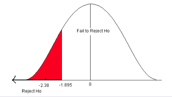
The critical value comes from the student’s t-distribution table with n – 1 degrees of freedom. In this problem, we have eight pairs of data (n = 8) with 7 degrees of freedom. This is a one-sided test (less than), so alpha is all in the left tail. Go down the 0.05 column with 7 df to find the correct critical value (tα) of -1.895.
3) The test statistic \[t=\frac {\bar {d}-\mu_{d}}{s_{d}/\sqrt {n}} = \frac {-5.125-0}{6.081/\sqrt{8}} = -2.38\]
We subtract zero from d-bar because of our null hypothesis. Our null hypothesis is that the difference of the before and after values are statistically equal to zero. In other words, there has been no change in water clarity.
4) Compare the test statistic to the critical value and state a conclusion.
The test statistic (-2.38) is less than the critical value (-1.895). It falls in the rejection zone.

We reject the null hypothesis. We have enough evidence to support the claim that the mean water clarity has improved.
P-value Approach
We can also use the p-value approach to answer the question. To estimate p-value using the student’s t-table, go across the row for 7 degrees of freedom until you find the two values that the absolute value of your test statistic falls between.
Table 4. Student t-Distribution.
|
df |
.05 |
.025 |
.02 |
.01 |
.005 |
|---|---|---|---|---|---|
|
5 |
2.015 |
2.571 |
2.757 |
3.365 |
4.032 |
|
6 |
1.943 |
2.447 |
2.612 |
3.143 |
3.707 |
|
7 |
1.895 |
2.365 |
2.517 |
2.998 |
3.499 |
|
8 |
1.860 |
2.306 |
2.449 |
2.896 |
3.355 |
|
9 |
1.833 |
2.262 |
2.398 |
2.821 |
3.250 |
The p-value for this test statistic is greater than 0.02 and just less than 0.025. Compare this to the level of significance (alpha). The Decision Rule says that if the p-value is less than α, reject the null hypothesis. In this case, the p-value estimate (0.02 – 0.025) is less than the level of significance (0.05). Reject the null hypothesis. We have enough evidence to support the claim that the mean water clarity has improved.
BUT, what if you used a 1% level of significance? In this case, the p-value is NOT less than the level of significance ((0.02 – 0.025)>0.01). We would fail to reject the null hypothesis. There is NOT enough evidence to support the claim that the water clarity has improved. It is important to set the level of significance at the start of your research and report the p-value. Another researcher may interpret your findings differently, based on your reported p-value and their own selected level of significance.
Construct and Interpret a Confidence Interval about the Differences of the Data for Matched Pairs
A hypothesis test for matched pairs data is very similar to a one-sample t-test. BUT, we can answer the same question by constructing a confidence interval about the mean of the differences. This process is just like the confidence intervals from Chapter 2.
- Find the critical value.
- Compute the margin of error.
- Point estimate ± margin of error.
For matched pairs data, the critical value comes from the student’s t-distribution with n – 1 degrees of freedom. The margin of error uses the sample standard deviation of the differences (sd) and the point estimate is \(\bar {d}\), the mean of the differences.
For a (1 – α)*100% confidence interval for the mean of the differences
\[\bar d\pm t_{\frac{\alpha}{2}}(\frac {s_d}{\sqrt {n}})\]
Where \(t_{\frac {\alpha}{2}}\) is used because confidence intervals are always two-sided.
Let’s look at the biologist studying water clarity in Owasco Lake again. She wants to test the claim that water clarity has improved. We can answer this question by constructing a confidence interval about the mean of the differences.
|
d̄ = -5.125 |
sd = 6.081 |
α = 0.05 |
n = 8 |
Solution
1) \(t_{\frac {\alpha}{2}} = 2.365\)
2) \(E=t_{\frac {\alpha}{2}}(\frac {s_d}{\sqrt {n}})=2.365(\frac {6.081}{\sqrt {8}}) = 5.085\)
3) \(\bar {d} \pm E = -5.125 \pm 5.085\)
The 95% confidence interval about the mean of the differences is
\((-10.21, -0.04)\)
\((-10.21\le \mu_d \le -0.04)\)
We can be 95% confident that this interval contains the true mean of the differences in water clarity between the two time periods. BUT, this doesn’t directly answer the question about improved water clarity. To do this, we use the interpretations given below.
Confidence Interval Interpretations
- If the confidence interval contains all positive values, we find a significant difference between the groups, AND we can conclude that the mean of the first group is significantly greater than the mean of the second group.
- If the confidence interval contains all negative values, we find a significant difference between the groups, AND we can conclude that the mean of the first group is significantly less than the mean of the second group.
- If the confidence interval contains zero (it goes from negative to positive values), we find NO significant difference between the groups.
In this problem, the confidence interval is (-10.21, -0.04). We have all negative values, so we can conclude that there is a significant difference in the mean water clarity between the years AND…
- The mean water clarity for the initial time was significantly less than at the five-year re-measurement.
- Water clarity has improved during the five-year period. The confidence interval estimates the mean improvement.
Biologists are studying elk migration in the western US and want to know if the four-lane interstate that was built ten years ago has disturbed elk migration to the winter feeding area. A random sample was gathered from nine wilderness districts in the winter feeding areas. These data were compared to a random sample collected from the same nine areas before the highway was built. Use a 1% level of significance to test this claim.
|
District |
1 |
2 |
3 |
4 |
5 |
6 |
7 |
8 |
9 |
|---|---|---|---|---|---|---|---|---|---|
|
Before |
11.6 |
18.7 |
15.9 |
20.6 |
10.1 |
17.4 |
7.2 |
12.2 |
11.7 |
|
After |
10.0 |
21.6 |
13.9 |
22.8 |
11.5 |
16.2 |
8.1 |
10.8 |
9.6 |
|
d |
1.6 |
-2.9 |
2.0 |
-2.2 |
-1.4 |
1.2 |
-0.9 |
1.4 |
2.1 |
\[\bar {d} = 0.100\]
\[s_d = 1.946\]
\(H_0: \mu_d = 0\)
\(H_1: \mu_d \ne 0\)
Determine the critical values: This is a two-sided question (alternative ≠) so the critical values are ±3.355.
Compute the test statistic:
\[t=\frac {\bar d -\mu_d}{s_d/\sqrt {n}} = \frac {0.100-0}{1.946/\sqrt {9}}=0.1542\]
Now compare the critical value to the test statistic and state a conclusion. The test statistic is NOT greater than 3.355 or less than -3.355 (it doesn’t fall in the rejection zones). We fail to reject the null hypothesis. There is not enough evidence to support the claim that the highway has interfered with the elk migration (no difference before or after the highway).
Now construct a 99% confidence interval and answer the question.
1) \(t_{\frac {\alpha}{2}}\) = 3.355
2) \(E=t_{\frac {\alpha}{2}}(\frac {s_d}{\sqrt{n}}) =3.355(1.946/\sqrt{9})=2.176\)
3) \(\bar d \pm E = 0.100\pm 2.176\)
The 99% confidence interval about the difference of the means is: (-2.076, 2.276)
This confidence interval contains zero. The null hypothesis is that there is zero difference before and after the highway way was created. Therefore, we fail to reject the null hypothesis. There is not enough evidence to support the claim that the highway has interfered with the elk migration (no difference before or after the highway).
Software Solutions
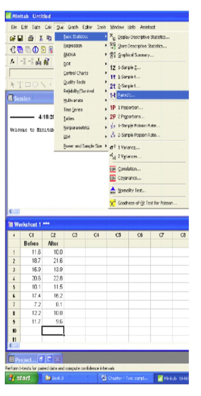
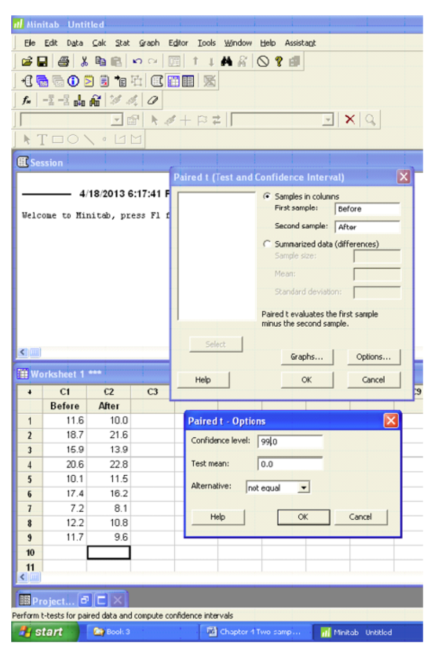
Minitab


Paired T-Test and CI: Before, After
|
N |
Mean |
StDev |
SE Mean |
|
|---|---|---|---|---|
|
Before |
9 |
13.93 |
4.42 |
1.47 |
|
After |
9 |
13.83 |
5.32 |
1.77 |
|
Difference |
9 |
0.100 |
1.946 |
0.649 |
|
99% CI for mean difference: (-2.077, 2.277) |
||||
|
T-Test of mean difference = 0 (vs not = 0): T-Value = 0.15 p-value = 0.881 |
||||
Minitab gives the test statistic of 0.15 and the p-value of 0.881. It also gives a 99% confidence interval for the difference of the means (-2.077, 2.277). All results support failing to reject the null hypothesis.
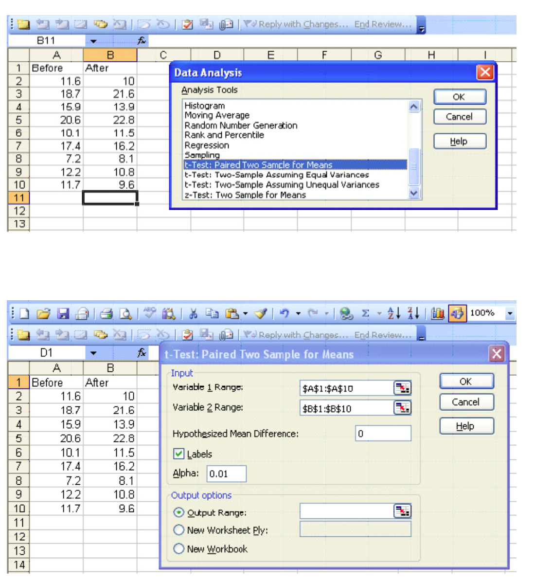
Excel

t-Test: Paired Two Sample for Means
|
Before |
After |
|
|---|---|---|
|
Mean |
13.93333 |
13.83333333 |
|
Variance |
19.565 |
28.3075 |
|
Observations |
9 |
9 |
|
Pearson Correlation |
0.936635 |
|
|
Hypothesized Mean Difference |
0 |
|
|
df |
8 |
|
|
t Stat |
0.15415 |
|
|
\(P(T\le t)\) one-tail |
0.440654 |
|
|
t Critical one-tail |
2.896459 |
|
|
\(P(T\le t)\) two-tail |
0.881309 |
|
|
t Critical two-tail |
3.355387 |
The test statistic is 0.15415. This is a two-sided question so we can use \(P(T\le t)\) two-tail = 0.881309. The p-value is NOT less than the 1% level of significance so we will fail to reject the null hypothesis.


