
19.3: Monte Carlo methods
- Page ID
- 45267

\( \newcommand{\vecs}[1]{\overset { \scriptstyle \rightharpoonup} {\mathbf{#1}} } \)
\( \newcommand{\vecd}[1]{\overset{-\!-\!\rightharpoonup}{\vphantom{a}\smash {#1}}} \)
\( \newcommand{\dsum}{\displaystyle\sum\limits} \)
\( \newcommand{\dint}{\displaystyle\int\limits} \)
\( \newcommand{\dlim}{\displaystyle\lim\limits} \)
\( \newcommand{\id}{\mathrm{id}}\) \( \newcommand{\Span}{\mathrm{span}}\)
( \newcommand{\kernel}{\mathrm{null}\,}\) \( \newcommand{\range}{\mathrm{range}\,}\)
\( \newcommand{\RealPart}{\mathrm{Re}}\) \( \newcommand{\ImaginaryPart}{\mathrm{Im}}\)
\( \newcommand{\Argument}{\mathrm{Arg}}\) \( \newcommand{\norm}[1]{\| #1 \|}\)
\( \newcommand{\inner}[2]{\langle #1, #2 \rangle}\)
\( \newcommand{\Span}{\mathrm{span}}\)
\( \newcommand{\id}{\mathrm{id}}\)
\( \newcommand{\Span}{\mathrm{span}}\)
\( \newcommand{\kernel}{\mathrm{null}\,}\)
\( \newcommand{\range}{\mathrm{range}\,}\)
\( \newcommand{\RealPart}{\mathrm{Re}}\)
\( \newcommand{\ImaginaryPart}{\mathrm{Im}}\)
\( \newcommand{\Argument}{\mathrm{Arg}}\)
\( \newcommand{\norm}[1]{\| #1 \|}\)
\( \newcommand{\inner}[2]{\langle #1, #2 \rangle}\)
\( \newcommand{\Span}{\mathrm{span}}\) \( \newcommand{\AA}{\unicode[.8,0]{x212B}}\)
\( \newcommand{\vectorA}[1]{\vec{#1}} % arrow\)
\( \newcommand{\vectorAt}[1]{\vec{\text{#1}}} % arrow\)
\( \newcommand{\vectorB}[1]{\overset { \scriptstyle \rightharpoonup} {\mathbf{#1}} } \)
\( \newcommand{\vectorC}[1]{\textbf{#1}} \)
\( \newcommand{\vectorD}[1]{\overrightarrow{#1}} \)
\( \newcommand{\vectorDt}[1]{\overrightarrow{\text{#1}}} \)
\( \newcommand{\vectE}[1]{\overset{-\!-\!\rightharpoonup}{\vphantom{a}\smash{\mathbf {#1}}}} \)
\( \newcommand{\vecs}[1]{\overset { \scriptstyle \rightharpoonup} {\mathbf{#1}} } \)
\(\newcommand{\longvect}{\overrightarrow}\)
\( \newcommand{\vecd}[1]{\overset{-\!-\!\rightharpoonup}{\vphantom{a}\smash {#1}}} \)
\(\newcommand{\avec}{\mathbf a}\) \(\newcommand{\bvec}{\mathbf b}\) \(\newcommand{\cvec}{\mathbf c}\) \(\newcommand{\dvec}{\mathbf d}\) \(\newcommand{\dtil}{\widetilde{\mathbf d}}\) \(\newcommand{\evec}{\mathbf e}\) \(\newcommand{\fvec}{\mathbf f}\) \(\newcommand{\nvec}{\mathbf n}\) \(\newcommand{\pvec}{\mathbf p}\) \(\newcommand{\qvec}{\mathbf q}\) \(\newcommand{\svec}{\mathbf s}\) \(\newcommand{\tvec}{\mathbf t}\) \(\newcommand{\uvec}{\mathbf u}\) \(\newcommand{\vvec}{\mathbf v}\) \(\newcommand{\wvec}{\mathbf w}\) \(\newcommand{\xvec}{\mathbf x}\) \(\newcommand{\yvec}{\mathbf y}\) \(\newcommand{\zvec}{\mathbf z}\) \(\newcommand{\rvec}{\mathbf r}\) \(\newcommand{\mvec}{\mathbf m}\) \(\newcommand{\zerovec}{\mathbf 0}\) \(\newcommand{\onevec}{\mathbf 1}\) \(\newcommand{\real}{\mathbb R}\) \(\newcommand{\twovec}[2]{\left[\begin{array}{r}#1 \\ #2 \end{array}\right]}\) \(\newcommand{\ctwovec}[2]{\left[\begin{array}{c}#1 \\ #2 \end{array}\right]}\) \(\newcommand{\threevec}[3]{\left[\begin{array}{r}#1 \\ #2 \\ #3 \end{array}\right]}\) \(\newcommand{\cthreevec}[3]{\left[\begin{array}{c}#1 \\ #2 \\ #3 \end{array}\right]}\) \(\newcommand{\fourvec}[4]{\left[\begin{array}{r}#1 \\ #2 \\ #3 \\ #4 \end{array}\right]}\) \(\newcommand{\cfourvec}[4]{\left[\begin{array}{c}#1 \\ #2 \\ #3 \\ #4 \end{array}\right]}\) \(\newcommand{\fivevec}[5]{\left[\begin{array}{r}#1 \\ #2 \\ #3 \\ #4 \\ #5 \\ \end{array}\right]}\) \(\newcommand{\cfivevec}[5]{\left[\begin{array}{c}#1 \\ #2 \\ #3 \\ #4 \\ #5 \\ \end{array}\right]}\) \(\newcommand{\mattwo}[4]{\left[\begin{array}{rr}#1 \amp #2 \\ #3 \amp #4 \\ \end{array}\right]}\) \(\newcommand{\laspan}[1]{\text{Span}\{#1\}}\) \(\newcommand{\bcal}{\cal B}\) \(\newcommand{\ccal}{\cal C}\) \(\newcommand{\scal}{\cal S}\) \(\newcommand{\wcal}{\cal W}\) \(\newcommand{\ecal}{\cal E}\) \(\newcommand{\coords}[2]{\left\{#1\right\}_{#2}}\) \(\newcommand{\gray}[1]{\color{gray}{#1}}\) \(\newcommand{\lgray}[1]{\color{lightgray}{#1}}\) \(\newcommand{\rank}{\operatorname{rank}}\) \(\newcommand{\row}{\text{Row}}\) \(\newcommand{\col}{\text{Col}}\) \(\renewcommand{\row}{\text{Row}}\) \(\newcommand{\nul}{\text{Nul}}\) \(\newcommand{\var}{\text{Var}}\) \(\newcommand{\corr}{\text{corr}}\) \(\newcommand{\len}[1]{\left|#1\right|}\) \(\newcommand{\bbar}{\overline{\bvec}}\) \(\newcommand{\bhat}{\widehat{\bvec}}\) \(\newcommand{\bperp}{\bvec^\perp}\) \(\newcommand{\xhat}{\widehat{\xvec}}\) \(\newcommand{\vhat}{\widehat{\vvec}}\) \(\newcommand{\uhat}{\widehat{\uvec}}\) \(\newcommand{\what}{\widehat{\wvec}}\) \(\newcommand{\Sighat}{\widehat{\Sigma}}\) \(\newcommand{\lt}{<}\) \(\newcommand{\gt}{>}\) \(\newcommand{\amp}{&}\) \(\definecolor{fillinmathshade}{gray}{0.9}\)edits: — under construction —
Introduction
Statistical methods that employ Monte Carlo methods use repeated random sampling to estimate properties of a frequency distribution. These distributions may be well-known, e.g., gamma-distribution, normal distribution, or \(t\)-distribution. The simulation is based on generation of a set of random numbers on the open interval \((0,1)\) — the set of real numbers between zero and one (all numbers greater than 0 and less than 1).
If the set included 0 and 1, then it would be called a closed set, i.e., the set includes the boundary points zero and one.
The Markov chain Monte Carlo (MCMC) sampling approach can be used to solve large scale problems. The Markov chain refers to how the sample is drawn from a specified probability distribution. It can be drawn by discrete time steps (DTMC) or by a continuous process (CTMC). The Markov process is “memoryless:” predictions of future events are derived solely from their present state — the future and past states are independent.
Gibbs sampling is a common MCMC algorithm.
R code
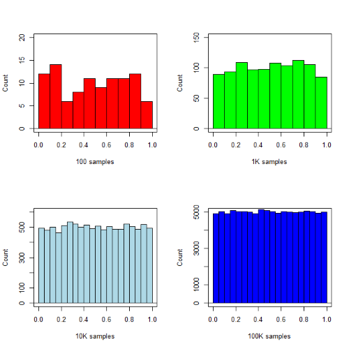
R’s uniform generator is runif function. Examples of the samples generated over different values (100, 1000, 10000, 100000) with output displayed as histograms (Fig. 1). Note that as sample size increases, the simulated distributions resemble more and more the uniform distribution. Use set.seed() to reproduce the same set and sequence of numbers
require(RcmdrMisc)
par(mfrow = c(2, 2))
myUniformH <- data.frame(runif(100))
with(myUniformH, Hist(runif.100., scale="frequency", ylim=c(0,20), breaks="Sturges", col="red", xlab="100 samples", ylab="Count"))
myUniform1K <- data.frame(runif(1000))
with(myUniform1K, Hist(runif.1000., scale="frequency", ylim=c(0,150), breaks="Sturges", col="green", xlab="1K samples", ylab="Count"))
myUniform10K <- data.frame(runif(10000))
with(myUniform10K, Hist(runif.10000., scale="frequency", ylim=c(0,600), breaks="Sturges", col="lightblue", xlab="10K samples", ylab="Count"))
myUniform100K <- data.frame(runif(100000))
with(myUniform100K, Hist(runif.100000., scale="frequency", ylim=c(0,5000),breaks="Sturges", col="blue", xlab="100K samples", ylab="Count"))
#reset par()
dev.off()
Yes, a nice repeating function would be more elegant code, but we move on. As a suggestion, you should create one! Use sapply() or a basic for loop.
Looks pretty uniform. A property of random numbers is that history should not influence the future, i.e., no autocorrelation. We can check using the acf() function (Fig. \(\PageIndex{2}\)).
par(mfrow = c(2, 2))
acf(myUniformH, main="100")
acf(myUniform1K, main="1K")
acf(myUniform10K, main="10K")
acf(myUniform100K, main="100K"
dev.off()
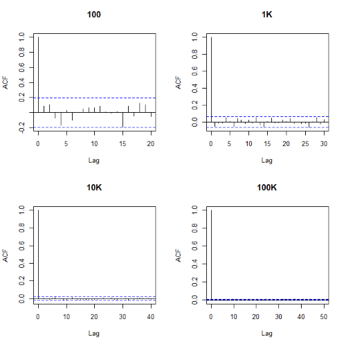
Correlations among points are plotted versus lag, where lag refers to the number of points between adjacent points, e.g., lag = 10 reflects the correlation among points 1 and 11, 2 and 12, and so forth. The band defined by two parallel blue dashed lines
Questions
- Use
set.seed(123)and repeatrunif(10)twice. Confirm that the two sets are different (do not set seed) or the same whenset.seedis used. R hint: use functionidentical(x,y), where x and y are the two generated samples. This function tests whether the values and sequence of elements are the same between the two vectors.