8.6: Confidence limits for the estimate of population mean

Introduction

In Chapter 3.4 and Chapter 8.3, we introduced the concept of providing a confidence interval for estimates. We gave a calculation for an approximate confidence interval for proportions and for the Number Needed to Treat (Chapter 7.3). Even an approximate confidence interval gives the reader a range of possible values of a population parameter from a sample of observations.

In this chapter we review and expand how to calculate the confidence interval for a sample mean, \(\bar{X}\). Because \(\bar{X}\) is derived from a sample of observations, we use the \(t\)-distribution to calculate the confidence interval. Note that if the population was known (population standard deviation), then you would use normal distribution. This was the basis for our recommendation to adjust your very approximate estimate of a confidence interval for an estimate by replacing the “2” with “1.96” when you multiply the standard error of the estimate \((SE)\) in the equation estimate \(\bar{X} \pm 2 \cdot SE\). As you can imagine, the approximation works for large sample size, but is less useful as sample size decreases.

Consider \(\bar{X}\); it is a point estimate of \(\mu\), the population mean (a parameter). But our estimate of \(\bar{X}\) is but one of an infinite number of possible estimates. The confidence interval, however, gives us a way to communicate how reliable our estimate is for the population parameter. A 95% confidence interval, for example, tells the reader that we are willing to say (95% confident) the true value of the parameter is between these two numbers (a lower limit and an upper limit). The point estimate (the sample mean) will of course be included between the two limits.

Instead of 95% confidence, we could calculate intervals for 99%. Since 99% is greater than 95%, we would communicate our certainty of our estimate.

Note

Again, the caveats about p-value extend to confidence intervals. See Chapter 8.2.

Question 1: For 99% confidence interval, the lower limit would be smaller than the lower limit for a 95% confidence interval.

1. True \(\color{Red} \leftarrow \text{Answer}\)
2. False

When we set the Type I error rate, \(\alpha\) (alpha) = 0.05 (5%), that means that 5% of all possible sample means from a population with mean, \(\mu\), will result in \(t\) values that are larger than \(+t_{0.05(2), df}\) OR smaller than \(-t_{0.05(2), df}\).

Why the \(t\)-distribution?

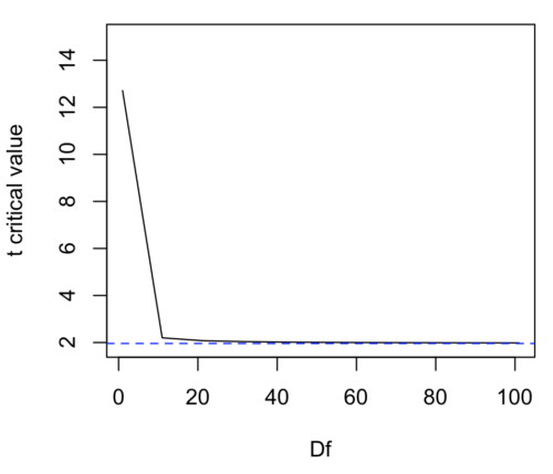
We use the \(t\)-test because, technically, we have a limited sample size and the \(t\)-distribution is more accurate than the normal distribution for small samples. Note that as sample size increases, the \(t\)-distribution is not distinguishable from the normal distribution and we could use \(\pm 1.96\) (Fig. \(\PageIndex{1}\)).

Figure \(\PageIndex{1}\): Copy and Paste Caption here. (Copyright; author via source)

Here’s the equation for calculating the confidence interval based on the t-distribution. These set the limits around our estimate of the sample mean. Together, they’re called the 95% confidence interval, \(1 - 0.05 = 0.95\).

\[P \left[-t_{0.05 \left(2 \right), df} \leq \frac{\bar{X}-\mu}{s_{\bar{X}}} \leq + t_{0.05 \left(2\right), df}\right] = 0.95 \nonumber\]

Here’s a simplified version of the same thing, but generalized to any Type I level…

\[\bar{X} \ \pm \ t_{\alpha/2, v} \cdot s_{\bar{X}} \nonumber\]

This statistic allows us to say that we are 95% confident that the interval \(\pm t_{0.05(2),df}\) includes the true value for \(\mu\). For this confidence interval you need to identify the critical \(t\) value at 5%. Thus, you need to know the degrees of freedom for this problem, which is simply \(n-1\), the sample size minus one.

It is straightforward to calculate these by hand, but…

Set the Type I error rate, calculate the degrees of freedom \((df)\):

• \(n - 1\) samples for one sample test
• \(n - 1\) pairs of samples for paired test
• \(n - 2\) samples for two independent sample test

and lookup the critical value from the t table (or from the \(t\) distribution in R). Of course, it is easier to use R.

In R, for the one tail critical value with seven degrees of freedom, type at the R prompt:

qt(c(0.05), df=7, lower.tail=FALSE)
[1] 1.894579

For the two-tail critical value:

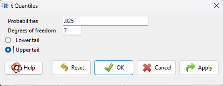
qt(c(0.025), df=7, lower.tail=FALSE)
[1] 2.364624

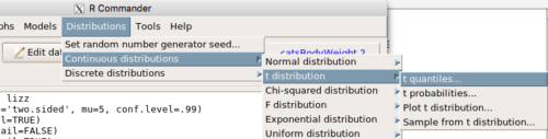
Or, if you prefer to use R Commander, then follow the menu prompts to bring up the t quantiles function (Fig. \(\PageIndex{2}\) and Fig. \(\PageIndex{3}\)).

Figure \(\PageIndex{2}\): Drop down menu to get \(t\)-distribution.

Note:

Quantiles divide probability distribution into equal parts or intervals. Quartiles have four groups, deciles have ten groups, and percentiles have 100 groups.

Figure \(\PageIndex{3}\): Menu for \(t\) quantiles, with values entered for the two-tail example.

You should confirm that what R calculates agrees with the critical values tabulated in the Table of Critical values for the t distribution provided in the Appendix.

A worked example

Let’s revisit our lizard example from last time (see Chapter 8.5). Prior to conducting any inference test, we decide acceptable Type I error rates (cf. justify alpha discussion in Chapter 8.1); For this example, we set Type I error rate to be 1% for a 99% confidence interval.

The Rcmdr output was

t.test(lizz$bm, alternative='two.sided', mu=5, conf.level=.99)
data: lizz$bm
t = -1.5079, df = 7, p-value = 0.1753
alternative hypothesis: true mean is not equal to 5 
99 percent confidence interval:
1.984737 6.199263
sample estimates:
mean of x
4.092

Sort through the output and identify what you need to know.

Question 1: What was the sample mean?

1. 5
2. -1.5079
3. 7
4. 0.1753
5. 1.984737
6. 6.199263
7. 4.092 \(\color{Red} \leftarrow \text{Answer}\)

Question 2: What was the most likely population mean?

1. 5 \(\color{Red} \leftarrow \text{Answer}\)
2. -1.5079
3. 7
4. 0.1753
5. 1.984737
6. 6.199263
7. 4.092

Question 3: This was a “one-tailed” test of the null hypothesis?

1. True
2. False \(\color{Red} \leftarrow \text{Answer}\)

The output states “alternative hypothesis: true mean is not equal to 5” — so it was a two-tailed test.

The 99% confidence interval \(\left(CI_{99\%}\right)\) is \((1.984737, 6.199263)\), which means we are 99% certain that the population mean is between 1.984737 (lower limit) and 6.199263 (the upper limit). In Chapter 8.5 we calculated the \(\left(CI_{95\%}\right)\) as \((2.667, 5.517)\).

Confidence intervals by nonparametric bootstrap sampling

Bootstrapping is a general approach to estimation or statistical inference that utilizes random sampling with replacement (Kulesa et al. 2015). In classic frequentist approach, a sample is drawn at random from the population and assumptions about the population distribution are made in order to conduct statistical inference. By resampling with replacement from the sample many times, the bootstrap samples can be viewed as if we drew from the population many times without invoking a theoretical distribution. A clear advantage of the bootstrap is that it allows estimation of confidence intervals without assuming a particular theoretical distribution and thus avoids the burden of repeating the experiment. Which method to prefer? For cases where assumption of a particular distribution is unwarranted (e.g., what is the appropriate distribution when we compare medians among samples?), bootstrap may be preferred (and for small data sets, percentile bootstrap may be better). We cover bootstrap sampling of confidence intervals in Chapter 19.2: Bootstrap sampling.

Conclusions

The take home message is simple.

• All estimates must be accompanied by a Confidence Interval.
• The more confident we wish to be, the wider the confidence interval will be.

Note that the confidence interval concept combines DESCRIPTION (the population mean is between these limits) and INFERENCE (and we are 95% certain about the values of these limits). It is good statistical practice to include estimates of confidence intervals for any estimate you share with readers. Any statistic that can be estimated should be accompanied by a confidence interval and, as you can imagine, formulas are available to do just this. For example, earlier this semester we calculated NNT.

---

Questions

1. Note in the worked example we used Type I error rate of 1%, not 5%. With a Type I error rate of 5% and sample size of 10, what will be the degrees of freedom \((df)\) for the \(t\) distribution?
2. Considering the information in question 1, what will be the critical value of the \(t\)-distribution for
   • a one-tailed test?
   • a two-tailed test
3. To gain practice with calculations of confidence intervals, calculate the approximate confidence interval, the 95% and the 99% confidence intervals based on the t distribution, for each of the following.

• • \(\bar{X} = 13\), \(s = 1.3\), \(n = 10\)
  • \(\bar{X} = 13\), \(s = 1.3\), \(n = 30\)
  • \(\bar{X} = 13\), \(s = 2.6\), \(n = 10\)
  • \(\bar{X} = 13\), \(s = 2.6\), \(n = 30\)

4. Take at look at your answers to question 3 — what trend(s) in the confidence interval calculations do you see with respect to variability?
5. Take at look at your answers to question 3 — what trend(s) in the confidence interval calculations do you see with respect to sample size?