
19.2: Bootstrap sampling
- Page ID
- 45266

\( \newcommand{\vecs}[1]{\overset { \scriptstyle \rightharpoonup} {\mathbf{#1}} } \)
\( \newcommand{\vecd}[1]{\overset{-\!-\!\rightharpoonup}{\vphantom{a}\smash {#1}}} \)
\( \newcommand{\dsum}{\displaystyle\sum\limits} \)
\( \newcommand{\dint}{\displaystyle\int\limits} \)
\( \newcommand{\dlim}{\displaystyle\lim\limits} \)
\( \newcommand{\id}{\mathrm{id}}\) \( \newcommand{\Span}{\mathrm{span}}\)
( \newcommand{\kernel}{\mathrm{null}\,}\) \( \newcommand{\range}{\mathrm{range}\,}\)
\( \newcommand{\RealPart}{\mathrm{Re}}\) \( \newcommand{\ImaginaryPart}{\mathrm{Im}}\)
\( \newcommand{\Argument}{\mathrm{Arg}}\) \( \newcommand{\norm}[1]{\| #1 \|}\)
\( \newcommand{\inner}[2]{\langle #1, #2 \rangle}\)
\( \newcommand{\Span}{\mathrm{span}}\)
\( \newcommand{\id}{\mathrm{id}}\)
\( \newcommand{\Span}{\mathrm{span}}\)
\( \newcommand{\kernel}{\mathrm{null}\,}\)
\( \newcommand{\range}{\mathrm{range}\,}\)
\( \newcommand{\RealPart}{\mathrm{Re}}\)
\( \newcommand{\ImaginaryPart}{\mathrm{Im}}\)
\( \newcommand{\Argument}{\mathrm{Arg}}\)
\( \newcommand{\norm}[1]{\| #1 \|}\)
\( \newcommand{\inner}[2]{\langle #1, #2 \rangle}\)
\( \newcommand{\Span}{\mathrm{span}}\) \( \newcommand{\AA}{\unicode[.8,0]{x212B}}\)
\( \newcommand{\vectorA}[1]{\vec{#1}} % arrow\)
\( \newcommand{\vectorAt}[1]{\vec{\text{#1}}} % arrow\)
\( \newcommand{\vectorB}[1]{\overset { \scriptstyle \rightharpoonup} {\mathbf{#1}} } \)
\( \newcommand{\vectorC}[1]{\textbf{#1}} \)
\( \newcommand{\vectorD}[1]{\overrightarrow{#1}} \)
\( \newcommand{\vectorDt}[1]{\overrightarrow{\text{#1}}} \)
\( \newcommand{\vectE}[1]{\overset{-\!-\!\rightharpoonup}{\vphantom{a}\smash{\mathbf {#1}}}} \)
\( \newcommand{\vecs}[1]{\overset { \scriptstyle \rightharpoonup} {\mathbf{#1}} } \)
\(\newcommand{\longvect}{\overrightarrow}\)
\( \newcommand{\vecd}[1]{\overset{-\!-\!\rightharpoonup}{\vphantom{a}\smash {#1}}} \)
\(\newcommand{\avec}{\mathbf a}\) \(\newcommand{\bvec}{\mathbf b}\) \(\newcommand{\cvec}{\mathbf c}\) \(\newcommand{\dvec}{\mathbf d}\) \(\newcommand{\dtil}{\widetilde{\mathbf d}}\) \(\newcommand{\evec}{\mathbf e}\) \(\newcommand{\fvec}{\mathbf f}\) \(\newcommand{\nvec}{\mathbf n}\) \(\newcommand{\pvec}{\mathbf p}\) \(\newcommand{\qvec}{\mathbf q}\) \(\newcommand{\svec}{\mathbf s}\) \(\newcommand{\tvec}{\mathbf t}\) \(\newcommand{\uvec}{\mathbf u}\) \(\newcommand{\vvec}{\mathbf v}\) \(\newcommand{\wvec}{\mathbf w}\) \(\newcommand{\xvec}{\mathbf x}\) \(\newcommand{\yvec}{\mathbf y}\) \(\newcommand{\zvec}{\mathbf z}\) \(\newcommand{\rvec}{\mathbf r}\) \(\newcommand{\mvec}{\mathbf m}\) \(\newcommand{\zerovec}{\mathbf 0}\) \(\newcommand{\onevec}{\mathbf 1}\) \(\newcommand{\real}{\mathbb R}\) \(\newcommand{\twovec}[2]{\left[\begin{array}{r}#1 \\ #2 \end{array}\right]}\) \(\newcommand{\ctwovec}[2]{\left[\begin{array}{c}#1 \\ #2 \end{array}\right]}\) \(\newcommand{\threevec}[3]{\left[\begin{array}{r}#1 \\ #2 \\ #3 \end{array}\right]}\) \(\newcommand{\cthreevec}[3]{\left[\begin{array}{c}#1 \\ #2 \\ #3 \end{array}\right]}\) \(\newcommand{\fourvec}[4]{\left[\begin{array}{r}#1 \\ #2 \\ #3 \\ #4 \end{array}\right]}\) \(\newcommand{\cfourvec}[4]{\left[\begin{array}{c}#1 \\ #2 \\ #3 \\ #4 \end{array}\right]}\) \(\newcommand{\fivevec}[5]{\left[\begin{array}{r}#1 \\ #2 \\ #3 \\ #4 \\ #5 \\ \end{array}\right]}\) \(\newcommand{\cfivevec}[5]{\left[\begin{array}{c}#1 \\ #2 \\ #3 \\ #4 \\ #5 \\ \end{array}\right]}\) \(\newcommand{\mattwo}[4]{\left[\begin{array}{rr}#1 \amp #2 \\ #3 \amp #4 \\ \end{array}\right]}\) \(\newcommand{\laspan}[1]{\text{Span}\{#1\}}\) \(\newcommand{\bcal}{\cal B}\) \(\newcommand{\ccal}{\cal C}\) \(\newcommand{\scal}{\cal S}\) \(\newcommand{\wcal}{\cal W}\) \(\newcommand{\ecal}{\cal E}\) \(\newcommand{\coords}[2]{\left\{#1\right\}_{#2}}\) \(\newcommand{\gray}[1]{\color{gray}{#1}}\) \(\newcommand{\lgray}[1]{\color{lightgray}{#1}}\) \(\newcommand{\rank}{\operatorname{rank}}\) \(\newcommand{\row}{\text{Row}}\) \(\newcommand{\col}{\text{Col}}\) \(\renewcommand{\row}{\text{Row}}\) \(\newcommand{\nul}{\text{Nul}}\) \(\newcommand{\var}{\text{Var}}\) \(\newcommand{\corr}{\text{corr}}\) \(\newcommand{\len}[1]{\left|#1\right|}\) \(\newcommand{\bbar}{\overline{\bvec}}\) \(\newcommand{\bhat}{\widehat{\bvec}}\) \(\newcommand{\bperp}{\bvec^\perp}\) \(\newcommand{\xhat}{\widehat{\xvec}}\) \(\newcommand{\vhat}{\widehat{\vvec}}\) \(\newcommand{\uhat}{\widehat{\uvec}}\) \(\newcommand{\what}{\widehat{\wvec}}\) \(\newcommand{\Sighat}{\widehat{\Sigma}}\) \(\newcommand{\lt}{<}\) \(\newcommand{\gt}{>}\) \(\newcommand{\amp}{&}\) \(\definecolor{fillinmathshade}{gray}{0.9}\)Introduction
Bootstrapping is a general approach to estimation or statistical inference that utilizes random sampling with replacement (Kulesa et al. 2015). In classic frequentist approach, a sample is drawn at random from the population and assumptions about the population distribution are made in order to conduct statistical inference. By resampling with replacement from the sample many times, the bootstrap samples can be viewed as if we drew from the population many times without invoking a theoretical distribution. A clear advantage of the bootstrap is that it allows estimation of confidence intervals without assuming a particular theoretical distribution and thus avoids the burden of repeating the experiment.
Base install of R includes the boot package. The boot package allows R users to work with most functions, and many authors have provided helpful packages. I highlight a couple packages
install packages lmboot, confintr
Example data set, Tadpoles from Chapter 14, copied to end of this page for convenience (scroll down or click here).
Bootstrapped 95% Confidence interval of population mean
Recall the classic frequentist (large-sample) approach to confidence interval estimates of mean using R:
x = round(mean(Tadpole$Body.mass),2); x
n = length(Tadpole$Body.mass); n
s = sd(Tadpole$Body.mass); s
error = qt(0.975,df=n-1)*(s/sqrt(n)); error
lower_ci = round(x-error,3)
upper_ci = round(x+error,3)
paste("95% CI of ", x, " between:", lower_ci, "&", upper_ci)
Output results are
> n = length(Tadpole$Body.mass); n
[1] 13
> s = sd(Tadpole$Body.mass); s
[1] 0.6366207
> error = qt(0.975,df=n-1)*(s/sqrt(n)); error
[1] 0.384706
> paste("95% CI of ", x, " between:", lower_ci, "&", upper_ci)
[1] "95% CI of 2.41 between: 2.025 & 2.795"
We used the t-distribution because both \(\mu\), the population mean, and \(\sigma\), the population standard deviation, were unknown. Thus, 95 out of 100 confidence intervals would be expected to include the true value.
Bootstrap equivalent:
library(confintr)
ci_mean(Tadpole$Body.mass, type=c("bootstrap"), boot_type=c("stud"), R=999, probs=c(0.025, 0.975), seed=1)
Output results are
Two-sided 95% bootstrap confidence interval for the population mean based on 999 bootstrap replications
and the student method

Sample estimate: 2.412308
Confidence interval:
    2.5%    97.5%
2.075808 2.880144
where stud is short for student t distribution (another common option is the percentile method — replace stud with perc), R = 999 directs the function to resample 999 times. We set seed=1 to initialize the pseudorandom number generator so that if we run the command again, we would get the same result. Any integer number can be used. For example, I set seed = 1 for the output below:
Confidence interval:
    2.5%    97.5%
2.075808 2.880144
Compare it to repeated runs without initializing the pseudorandom number generator:
Confidence interval:
    2.5%    97.5%
2.067558 2.934055
and again
Confidence interval:
    2.5%    97.5%
2.067616 2.863158
Note that the classic confidence interval is narrower than the bootstrap estimate, in part because of the small sample size (i.e., not as accurate, does not actually achieve the nominal 95% coverage). Which to use? The sample size was small, just 13 tadpoles. Bootstrap samples were drawn from the original data set, thus it cannot make a small study more robust. The 999 samples can be thought as estimating the sampling distribution. If the assumptions of the \(t\)-distribution hold, then the classic approach would be preferred. For the Tadpole data set, Body.mass was approximately normally distributed (Anderson-Darling test = 0.21179, p-value = 0.8163). For cases where assumption of a particular distribution is unwarranted (e.g., what is the appropriate distribution when we compare medians among samples?), bootstrap may be preferred (and for small data sets, percentile bootstrap may be better). To complete the analysis, percentile bootstrap estimate of confidence interval are presented.
The R code
ci_mean(Tadpole$Body.mass, type=c("bootstrap"), boot_type=c("perc"), R=999, probs=c(0.025, 0.975), seed=1)
and the output
Two-sided 95% bootstrap confidence interval for the population mean, based on 999 bootstrap replications and the percent method:
Sample estimate: 2.412308
Confidence interval:
    2.5%    97.5%
2.076923 2.749231
In this case, the bootstrap percentile confidence interval is narrower than the frequentist approach.
Model coefficients by bootstrap
R code
Enter the model, then set B, the number of samples with replacement.
myBoot <- residual.boot(VO2~Body.mass, B = 1000, data = Tadpoles)
R returns two values:
bootEstParam, which are the bootstrap parameter estimates. Each column in the matrix lists the values for a coefficient. For this model,bootEstParam$[,1]is the intercept andbootEstParam$[,2]is the slope.origEstParam, a vector with the original parameter estimates for the model coefficients.seed, numerical value for the seed; use seed number to get reproducible results. If you don’t specify the seed, then seed is set to pick any random number.
While you can list the $bootEstParam, not advisable because it will be a list of 1000 numbers (the value set with B)!
Get necessary statistics and plots
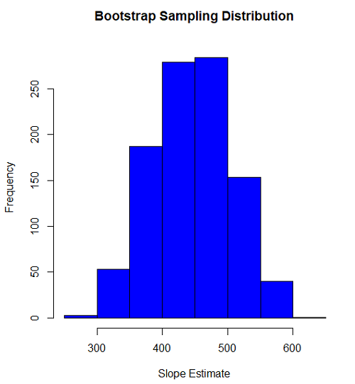
#95% CI slope
quantile(myBoot$bootEstParam[,2], probs=c(.025, .975))
R returns
    2.5%    97.5%
335.0000 562.6228
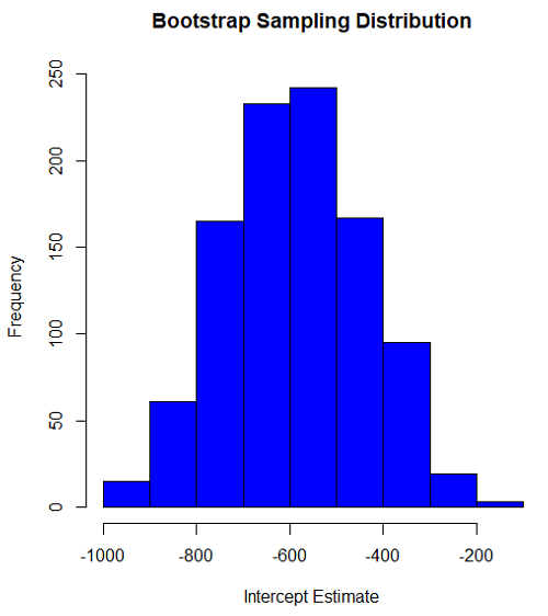
#95% CI intercept
quantile(myBoot$bootEstParam[,1], probs=c(.025, .975))
R returns
     2.5%     97.5%
-881.3893 -310.8209
Slope
#plot the sampling distribution of the slope coefficient
par(mar=c(5,5,5,5)) #setting margins to my preferred values
hist(myBoot$bootEstParam[,2], col="blue", main="Bootstrap Sampling Distribution",
xlab="Slope Estimate")
Intercept
#95% CI intercept
quantile(myBoot$bootEstParam[,1], probs=c(.025, .975))
par(mar=c(5,5,5,5))
hist(myBoot$bootEstParam[,1], col="blue", main="Bootstrap Sampling Distribution",
xlab="Intercept Estimate")
Questions
edits: pending
Data set used in this page (sorted)
| Gosner | Body mass | VO2 |
| I | 1.76 | 109.41 |
| I | 1.88 | 329.06 |
| I | 1.95 | 82.35 |
| I | 2.13 | 198 |
| I | 2.26 | 607.7 |
| II | 2.28 | 362.71 |
| II | 2.35 | 556.6 |
| II | 2.62 | 612.93 |
| II | 2.77 | 514.02 |
| II | 2.97 | 961.01 |
| II | 3.14 | 892.41 |
| II | 3.79 | 976.97 |
| NA | 1.46 | 170.91 |