9.2: Measuring Goodness of Fit

Once we have constructed a regression model, it is natural to ask: how good is the model at explaining variation in our dependent variable? We can answer this question with a number of statistics that indicate model fit“. Basically, these statistics provide measures of the degree to which the estimated relationships account for the variance in the dependent variable, YY.

There are several ways to examine how well the model explains" the variance in YY. First, we can examine the covariance of XX and YY, which is a general measure of the sample variance for XX and YY. Then we can use a measure of sample correlation, which is the standardized measure of covariation. Both of these measures provide indicators of the degree to which variation in XX can account for variation in YY. Finally, we can examine R2R2, also know as the coefficient of determination, which is the standard measure of the goodness of fit for OLS models.

9.2.1 Sample Covariance and Correlations

The sample covariance for a simple regression model is defined as:

SXY=Σ(Xi−¯X)(Yi−¯Y)n−1(9.5)(9.5)SXY=Σ(Xi−X¯)(Yi−Y¯)n−1

Intuitively, this measure tells you, on average, whether a higher value of XX (relative to its mean) is associated with a higher or lower value of YY. Is the association negative or positive? Covariance can be obtained quite simply in R by using the the cov function.

Sxy <- cov(ds.omit$ideol, ds.omit$glbcc_risk)
Sxy

## [1] -3.137767

The problem with covariance is that its magnitude will be entirely dependent on the scales used to measure XX and YY. That is, it is non-standard, and its meaning will vary depending on what it is that is being measured. In order to compare sample covariation across different samples and different measures, we can use the sample correlation.

The sample correlation, rr, is found by dividing SXYSXY by the product of the standard deviations of XX, SXSX, and YY, SYSY.

r=SXYSXSY=Σ(Xi−¯X)(Yi−¯Y)√Σ(Xi−¯X)2Σ(Yi−¯Y)2(9.6)(9.6)r=SXYSXSY=Σ(Xi−X¯)(Yi−Y¯)Σ(Xi−X¯)2Σ(Yi−Y¯)2

To calculate this in R, we first make an object for SXSX and SYSY using the sd function.

Sx <- sd(ds.omit$ideol)
Sx

## [1] 1.7317

Sy <- sd(ds.omit$glbcc_risk)
Sy

## [1] 3.070227

Then to find rr:

r <- Sxy/(Sx*Sy)
r

## [1] -0.5901706

To check this we can use the cor function in R.

rbyR <- cor(ds.omit$ideol, ds.omit$glbcc_risk)
rbyR

## [1] -0.5901706

So what does the correlation coefficient mean? The values range from +1 to -1, with a value of +1 means there is a perfect positive relationship between XX and YY. Each increment of increase in XX is matched by a constant increase in YY – with all observations lining up neatly on a positive slope. A correlation coefficient of -1, or a perfect negative relationship, would indicate that each increment of increase in XX corresponds to a constant decrease in YY – or a negatively sloped line. A correlation coefficient of zero would describe no relationship between XX and YY.

9.2.2 Coefficient of Determination: R2R2

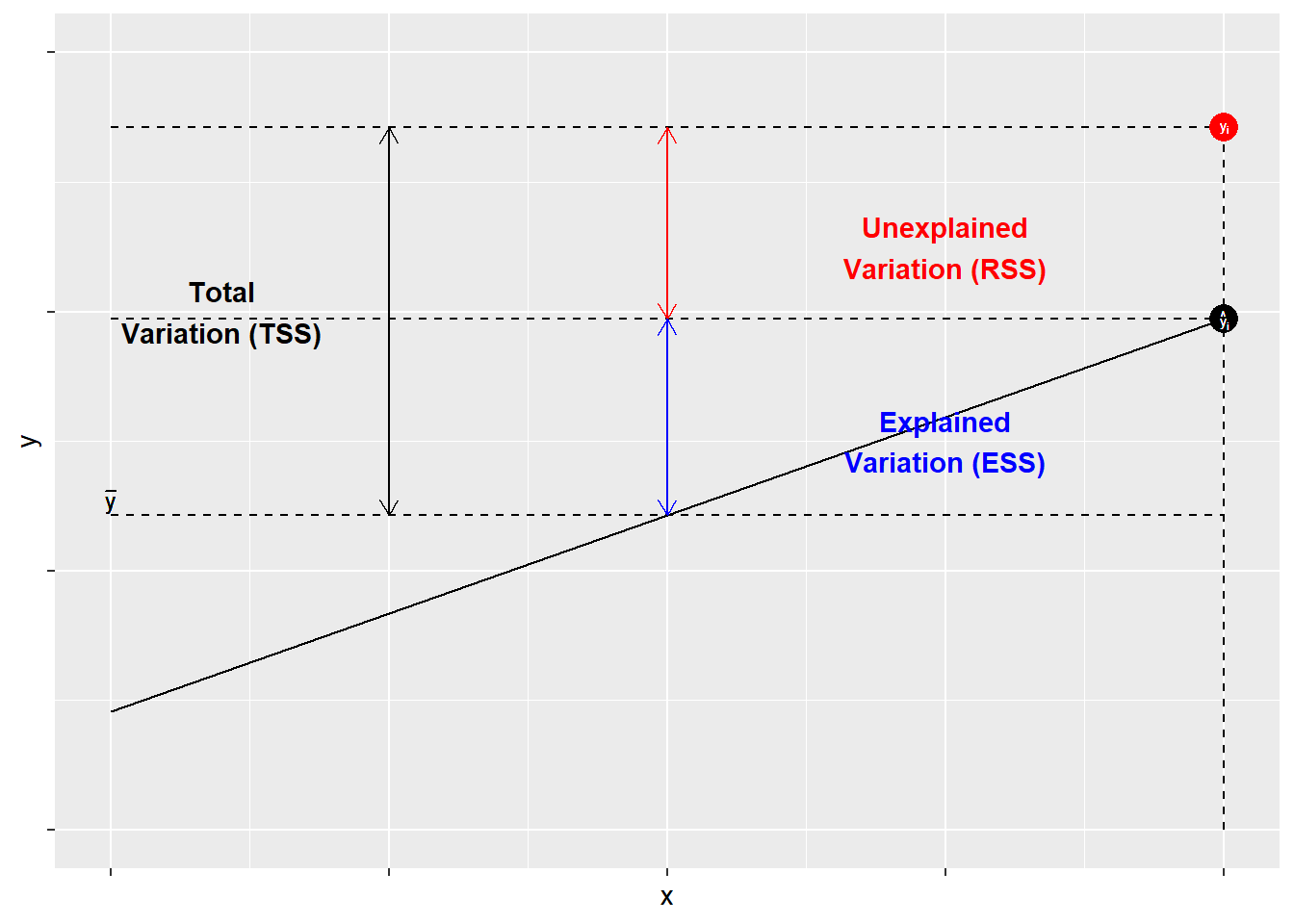
The most often used measure of goodness of fit for OLS models is R2R2. R2R2 is derived from three components: the total sum of squares, the explained sum of squares, and the residual sum of squares. R2R2 is the ratio of ESS (explained sum of squares) to TSS (total sum of squares).

Components of R2R2

• Total sum of squares (TSS): The sum of the squared variance of YY
• Residual sum of squares(RSS): The variance of YY not accounted for by the model
• Explained sum of squares (ESS): The variance of YY accounted for in the model. It is the difference between the TSS and the RSS.

• R2R2: The proportion of the total variance of YY explained by the model or the ratio of ESSESS to TSSTSS

R2=ESSTSS=TSS−RSSTSS=1−RSSTSSR2=ESSTSS=TSS−RSSTSS=1−RSSTSS

The components of R2R2 are illustrated in Figure \(\PageIndex{1}\). As shown, for each observation YiYi, variation around the mean can be decomposed into that which is “explained” by the regression and that which is not. In Figure \(\PageIndex{1}\), the deviation between the mean of YY and the predicted value of YY, ^YY^, is the proportion of the variation of YiYi that can be explained (or predicted) by the regression. That is shown as a blue line. The deviation of the observed value of YiYi from the predicted value ^YY^ (aka the residual, as discussed in the previous chapter) is the unexplained deviation, shown in red. Together, the explained and unexplained variation make up the total variation of YiYi around the mean ^YY^.

Figure \(\PageIndex{1}\): The Components of R2R2

To calculate R2R2 “by hand” in R, we must first determine the total sum of squares, which is the sum of the squared differences of the observed values of YY from the mean of YY, Σ(Yi−¯Y)2Σ(Yi−Y¯)2. Using R, we can create an object called TSS.

TSS <- sum((ds.omit$glbcc_risk-mean(ds.omit$glbcc_risk))^2)
TSS

## [1] 23678.85

Remember that R2R2 is the ratio of the explained sum of squares to the total sum of squares (ESS/TSS). Therefore to calculate R2R2 we need to create an object called RSS, the squared sum of our model residuals.

RSS <- sum(ols1$residuals^2)
RSS

## [1] 15431.48

Next, we create an object called ESS, which is equal to TSS-RSS.

ESS <- TSS-RSS
ESS

## [1] 8247.376

Finally, we calculate the R2R2.

R2 <- ESS/TSS
R2

## [1] 0.3483013

Note–happily–that the R2R2 calculated by “by hand” in R matches the results provided by the summary command.

The values for R2R2 can range from zero to 1. In the case of simple regression, a value of 1 indicates that the modeled coefficient (BB) “accounts for” all of the variation in YY. Put differently, all of the squared deviations in YiYi around the mean (^YY^) are in ESS, with none in the residual (RSS).¹⁶ A value of zero would indicate that all of the deviations in YiYi around the mean are in RSS – all residual or error“. Our example shows that the variation in political ideology (our XX) accounts for roughly 34.8 percent of the variation in our measure of the perceived risk of climate change (YY).

9.2.3 Visualizing Bivariate Regression

The ggplot2 the package provides a mechanism for viewing the effect of the independent variable, ideology, on the dependent variable, perceived risk of climate change. Adding geom_smooth will calculate and visualize a regression line that represents the relationship between your IV and DV while minimizing the residual sum of squares. Graphically (Figure \(\PageIndex{2}\)), we see as an individual becomes more conservative (ideology = 7), their perception of the risk of global warming decreases.

ggplot(ds.omit, aes(ideol, glbcc_risk)) +
  geom_smooth(method = lm)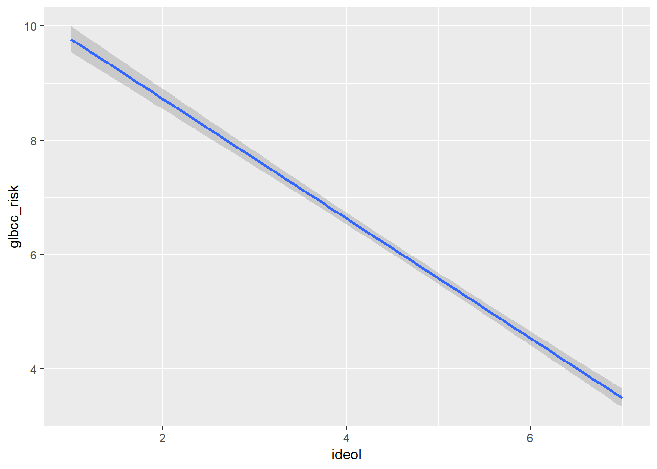

Figure \(\PageIndex{2}\): Bivariate Regression Plot

Cleaning up the R Environment

If you recall, at the beginning of the chapter, we created several temporary data sets. We should take the time to clear up our workspace for the next chapter. The rm function in R will remove them for us.

rm(ds.omit)