8.2: 8.2 Deriving OLS Estimators

Now that we have developed some of the rules for differential calculus, we can see how OLS finds values of ^αα^ and ^ββ^ that minimize the sum of the squared error. In formal terms, let’s define the set, S(^α,^β)S(α^,β^), as a pair of regression estimators that jointly determine the residual sum of squares given that: Yi=^Yi+ϵi=^α+^βXi+ϵiYi=Y^i+ϵi=α^+β^Xi+ϵi. This function can be expressed:

S(^α,^β)=n∑i=1ϵ2i=∑(Yi−^Yi)2=∑(Yi−^α−^βXi)2S(α^,β^)=∑i=1nϵi2=∑(Yi−Yi^)2=∑(Yi−α^−β^Xi)2

First, we will derive ^αα^.

8.2.1 OLS Derivation of ^αα^

Take the partial derivatives of S(^α,^β)S(α^,β^) with-respect-to (w.r.t) ^αα^ in order to determine the formulation of ^αα^ that minimizes S(^α,^β)S(α^,β^). Using the chain rule,

∂S(^α,^β)∂^α=∑2(Yi−^α−^βXi)2−1∗(Yi−^α−^βXi)′=∑2(Yi−^α−^βXi)1∗(−1)=−2∑(Yi−^α−^βXi)=−2∑Yi+2n^α+2^β∑Xi∂S(α^,β^)∂α^=∑2(Yi−α^−β^Xi)2−1∗(Yi−α^−β^Xi)′=∑2(Yi−α^−β^Xi)1∗(−1)=−2∑(Yi−α^−β^Xi)=−2∑Yi+2nα^+2β^∑Xi

Next, set the derivative equal to 00.

∂S(^α,^β)∂^α=−2∑Yi+2n^α+2^β∑Xi=0∂S(α^,β^)∂α^=−2∑Yi+2nα^+2β^∑Xi=0

Then, shift non-^αα^ terms to the other side of the equal sign:

2n^α=2∑Yi−2^β∑Xi2nα^=2∑Yi−2β^∑XiFinally, divide through by 2n2n:2n^α2n=2∑Yi−2^β∑Xi2nA=∑Yin−^β∗∑Xin=¯Y−^β¯X2nα^2n=2∑Yi−2β^∑Xi2nA=∑Yin−β^∗∑Xin=Y¯−β^X¯∴^α=¯Y−^β¯X(8.1)(8.1)∴α^=Y¯−β^X¯

8.2.2 OLS Derivation of ^ββ^

Having found ^αα^, the next step is to derive ^ββ^. This time we will take the partial derivative w.r.t ^ββ^. As you will see, the steps are a little more involved for ^ββ^ than they were for ^αα^.

∂S(^α,^β)∂^β=∑2(Yi−^α−^βXi)2−1∗(Yi−^α−^βXi)′=∑2(Yi−^α−^βXi)1∗(−Xi)=2∑(−XiYi+^αXi+^βX2i)=−2∑XiYi+2^α∑Xi+2^β∑X2i∂S(α^,β^)∂β^=∑2(Yi−α^−β^Xi)2−1∗(Yi−α^−β^Xi)′=∑2(Yi−α^−β^Xi)1∗(−Xi)=2∑(−XiYi+α^Xi+β^Xi2)=−2∑XiYi+2α^∑Xi+2β^∑Xi2

Since we know that ^α=¯Y−^β¯Xα^=Y¯−β^X¯, we can substitute ¯Y−^β¯XY¯−β^X¯ for ^αα^.

∂S(^α,^β)∂^β=−2∑XiYi+2(¯Y−^β¯X)∑Xi+2^β∑X2i=−2∑XiYi+2¯Y∑Xi−2^β¯X∑Xi+2^β∑X2i∂S(α^,β^)∂β^=−2∑XiYi+2(Y¯−β^X¯)∑Xi+2β^∑Xi2=−2∑XiYi+2Y¯∑Xi−2β^X¯∑Xi+2β^∑Xi2

Next, we can substitute ∑Yin∑Yin for ¯YY¯ and ∑Xin∑Xin for ¯XX¯ and set it equal to 00.

∂S(^α,^β)∂^β=−2∑XiYi+2∑Yi∑Xin−2^β∑Xi∑Xin+2^β∑X2i=0∂S(α^,β^)∂β^=−2∑XiYi+2∑Yi∑Xin−2β^∑Xi∑Xin+2β^∑Xi2=0

Then, multiply through by n2n2 and put all the ^ββ^ terms on the same side.

n^β∑X2i−^β(∑Xi)2=n∑XiYi−∑Xi∑Yi^β(n∑X2i−(∑Xi)2)=n∑XiYi−∑Xi∑Yi∴^β=n∑XiYi−∑Xi∑Yin∑X2i−(∑Xi)2nβ^∑Xi2−β^(∑Xi)2=n∑XiYi−∑Xi∑Yiβ^(n∑Xi2−(∑Xi)2)=n∑XiYi−∑Xi∑Yi∴β^=n∑XiYi−∑Xi∑Yin∑Xi2−(∑Xi)2

The ^ββ^ term can be rearranged such that:

^β=Σ(Xi−¯X)(Yi−¯Y)Σ(Xi−¯X)2(8.2)(8.2)β^=Σ(Xi−X¯)(Yi−Y¯)Σ(Xi−X¯)2

Now remember what we are doing here: we used the partial derivatives for ∑ϵ2∑ϵ2 with respect to ^αα^ and ^ββ^ to find the values for ^αα^ and ^ββ^ that will give us the smallest value for ∑ϵ2∑ϵ2. Put differently, the formulas for ^ββ^ and ^αα^ allow the calculation of the error-minimizing slope (change in YY given a one-unit change in XX) and intercept (value for YY when XX is zero) for any data set representing a bivariate, linear relationship. No other formulas will give us a line, using the same data, that will result in as small a squared-error. Therefore, OLS is referred to as the Best Linear Unbiased Estimator (BLUE).

8.2.3 Interpreting ^ββ^ and ^αα^

In a regression equation, Y=^α+^βXY=α^+β^X, where ^αα^ is shown in Equation (8.1) and ^ββ^ is shown in Equation (8.2). Equation (8.2) shows that for each 1-unit increase in XX you get ^ββ^ units to change in YY. Equation (8.1) shows that when XX is 00, YY is equal to ^αα^. Note that in a regression model with no independent variables, ^αα^ is simply the expected value (i.e., mean) of YY.

The intuition behind these formulas can be shown by using R to calculate “by hand” the slope (^ββ^) and intercept (^αα^) coefficients. A theoretical simple regression model is structured as follows:

Yi=α+βXi+ϵiYi=α+βXi+ϵi

• αα and ββ are constant terms
• αα is the intercept
• ββ is the slope
• XiXi is a predictor of YiYi
• ϵϵ is the error term

The model to be estimated is expressed as Y=^β+^βX+/epsilonY=β^+β^X+/epsilon.

As noted, the goal is to calculate the intercept coefficient:

^α=¯Y−^β¯Xα^=Y¯−β^X¯and the slope coefficient:^β=Σ(Xi−¯X)(Yi−¯Y)Σ(Xi−¯X)2β^=Σ(Xi−X¯)(Yi−Y¯)Σ(Xi−X¯)2

Using R, this can be accomplished in a few steps. First, create a vector of values for x and y (note that we chose these values arbitrarily for the purpose of this example).

x <- c(4,2,4,3,5,7,4,9)
x

## [1] 4 2 4 3 5 7 4 9

y <- c(2,1,5,3,6,4,2,7)
y

## [1] 2 1 5 3 6 4 2 7

Then, create objects for ¯XX¯ and ¯YY¯:

xbar <- mean(x)
xbar

## [1] 4.75

ybar <- mean(y)
ybar

## [1] 3.75

Next, create objects for (X−¯X)(X−X¯) and (Y−¯Y)(Y−Y¯), the deviations of XX and YY around their means:

x.m.xbar <- x-xbar
x.m.xbar

## [1] -0.75 -2.75 -0.75 -1.75  0.25  2.25 -0.75  4.25

y.m.ybar <- y-ybar
y.m.ybar

## [1] -1.75 -2.75  1.25 -0.75  2.25  0.25 -1.75  3.25

Then, calculate ^ββ^:

^β=Σ(Xi−¯X)(Yi−¯Y)Σ(Xi−¯X)2β^=Σ(Xi−X¯)(Yi−Y¯)Σ(Xi−X¯)2

B <- sum((x.m.xbar)*(y.m.ybar))/sum((x.m.xbar)^2)
B

## [1] 0.7183099

Finally, calculate ^αα^

^α=¯Y−^β¯Xα^=Y¯−β^X¯

A <- ybar-B*xbar
A

## [1] 0.3380282

To see the relationship, we can produce a scatterplot of x and y and add our regression line, as shown in Figure \(\PageIndex{4}\). So, for each unit increase in xx, yy increases by 0.7183099 and when xx is 00, yy is equal to 0.3380282.

plot(x,y)
lines(x,A+B*x)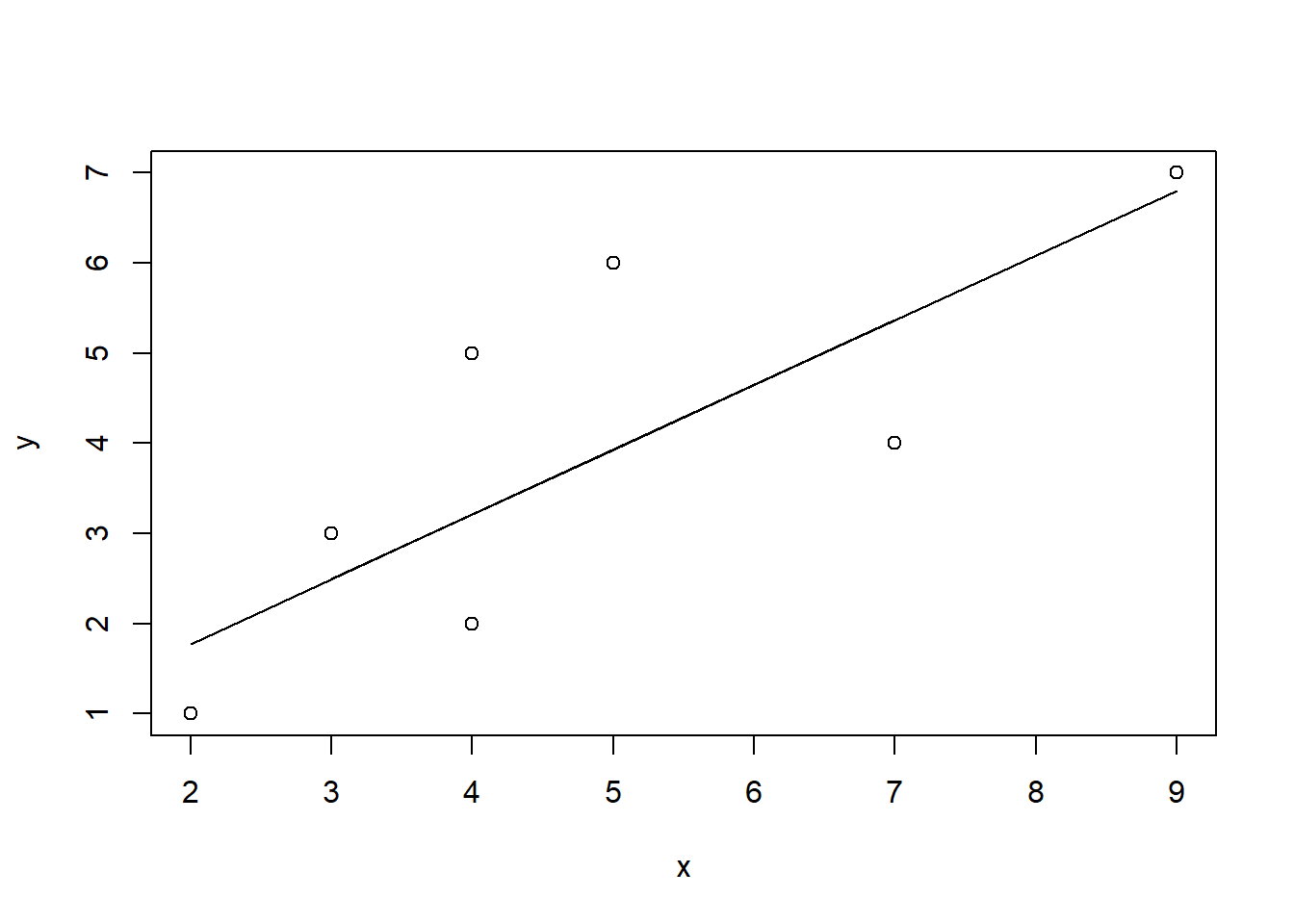

Figure \(\PageIndex{4}\): Simple Regression of xx and yy

dev.off()

## RStudioGD 
##         2