8.1: Minimizing Error using Derivatives

In calculus, the derivative is a measure of the slope of any function of x, or f(x)f(x), at each given value of xx. For the function f(x)f(x), the derivative is denoted as f′(x)f′(x) or, pronounced as “f prime x”. Because the formula for ∑ϵ2∑ϵ2 is known and can be treated as a function, the derivative of that function permits the calculation of the change in the sum of the squared error over each possible value of ^αα^ and ^ββ^. For that reason, we need to find the derivative for ∑ϵ2∑ϵ2 with respect to changes in ^αα^ and ^ββ^. That, in turn, will permit us to “derive” the values of ^αα^ and ^ββ^ that result in the lowest possible ∑ϵ2∑ϵ2.

Look – we understand that this all sounds complicated. But it’s not all that complicated. In this chapter, we will walk through all the steps so you’ll see that it's really rather simple and, well, elegant. You will see that differential calculus (the kind of calculus that is concerned with rates of change) is built on a set of clearly defined rules for finding the derivative for any function f(x)f(x). It’s like solving a puzzle. The next section outlines these rules, so we can start solving puzzles.

8.1.1 Rules of Derivation

Derivative Rules

1. Power Rule
2. Constant Rule
3. A Constant Times a Function
4. Differentiating a Sum
5. Product Rule
6. Quotient Rule
7. Chain Rule

The following sections provide examples of the application of each rule.

Rule 1: The Power Rule

Example:f(x)=x6f′(x)=6∗x6−1=6x5f(x)=x6f′(x)=6∗x6−1=6x5

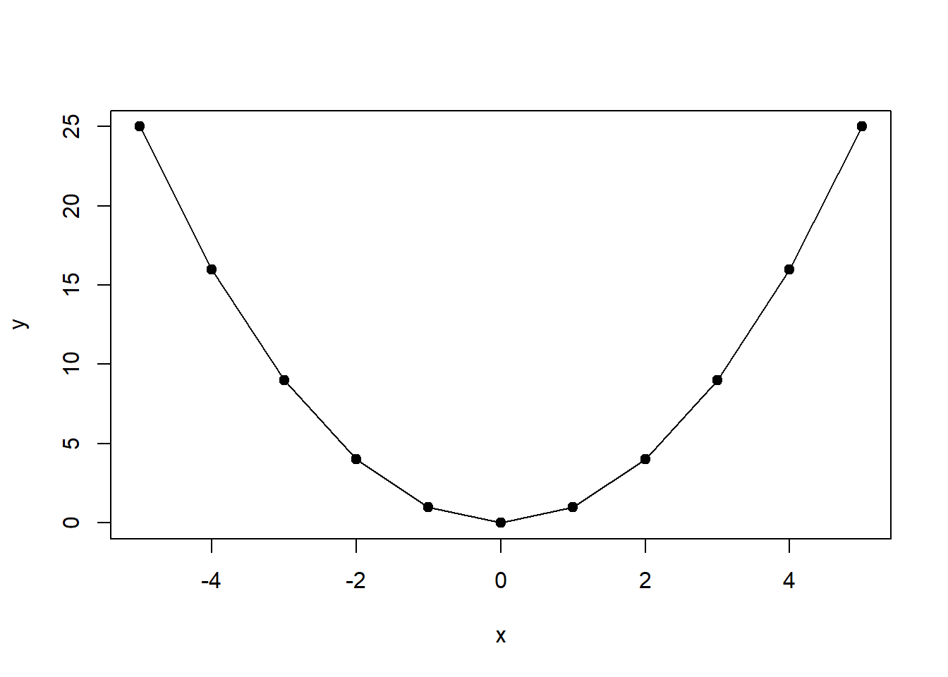
A second example can be plotted in R. The function is f(x)=x2f(x)=x2 and therefore, using the power rule, the derivative is: f′(x)=2xf′(x)=2x.

x <- c(-5:5)
x

##  [1] -5 -4 -3 -2 -1  0  1  2  3  4  5

y <- x^2
y

##  [1] 25 16  9  4  1  0  1  4  9 16 25

plot(x,y, type="o", pch=19)

Figure \(\PageIndex{1}\): Calculating Slopes for (x,y)(x,y) Pairs

Rule 2: The Constant Rule

Example:f(x)=346f′(x)=0=10xf(x)=346f′(x)=0=10x

Rule 3: A Constant Times a Function

Example:f(x)=5x2f′(x)=5∗2x2−1=10xf(x)=5x2f′(x)=5∗2x2−1=10x

Rule 4: Differentiating a Sum

Example:
f(x)=4x2+32xf′(x)=(4x2)′+(32x)′=4∗2x2−1+32=8x+32f(x)=4x2+32xf′(x)=(4x2)′+(32x)′=4∗2x2−1+32=8x+32

Rule 5: The Product Rule

Example:f(x)=x3(x−5)f′(x)=(x3)′(x−5)+(x3)(x−5)′=3x2(x−5)+(x3)∗1=3x3−15x2+x3=4x3−15x2f(x)=x3(x−5)f′(x)=(x3)′(x−5)+(x3)(x−5)′=3x2(x−5)+(x3)∗1=3x3−15x2+x3=4x3−15x2

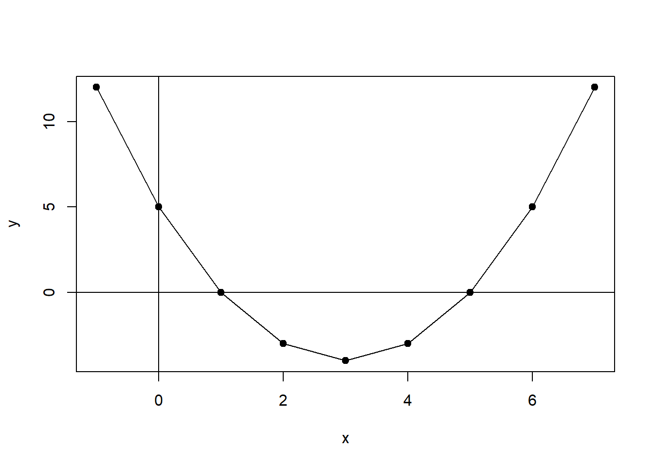
In a second example, the product rule is applied to the function y=f(x)=x2−6x+5y=f(x)=x2−6x+5. The derivative of this function is f′(x)=2x−6f′(x)=2x−6. This function can be plotted in R.

x <- c(-1:7)
x

## [1] -1  0  1  2  3  4  5  6  7

y <- x^2-6*x+5
y

## [1] 12  5  0 -3 -4 -3  0  5 12

plot(x,y, type="o", pch=19)
abline(h=0,v=0)

Figure \(\PageIndex{2}\): Plot of Function y=f(x)=x2−6x+5y=f(x)=x2−6x+5

We can also use the derivative and R to calculate the slope for each value of XX.

b <- 2*x-6
b

## [1] -8 -6 -4 -2  0  2  4  6  8

The values for XX, which are shown in Figure \(\PageIndex{2}\), range from -8 to +8 and return derivatives (slopes at a point) ranging from -25 to +25.

Rule 6: the Quotient Rule

Example:f(x)=xx2+5f′(x)=(x2+5)(x)′−(x2+5)′(x)(x2+5)2=(x2+5)−(2x)(x)(x2+5)2=−x2+5(x2+5)2f(x)=xx2+5f′(x)=(x2+5)(x)′−(x2+5)′(x)(x2+5)2=(x2+5)−(2x)(x)(x2+5)2=−x2+5(x2+5)2

Rule 7: The Chain Rule

Example:f(x)=(7x2−2x+13)5f′(x)=5(7x2−2x+13)4∗(7x2−2x+13)′=5(7x2−2x+13)4∗(14x−2)f(x)=(7x2−2x+13)5f′(x)=5(7x2−2x+13)4∗(7x2−2x+13)′=5(7x2−2x+13)4∗(14x−2)

8.1.2 Critical Points

Our goal is to use derivatives to find the values of ^αα^ and ^ββ^ that minimize the sum of the squared error. To do this we need to find the minima of a function. The minima is the smallest value that a function takes, whereas the maxima is the largest value. To find the minima and maxima, the critical points are key. The critical point is where the derivative of the function is equal to 00, or f′(x)=0f′(x)=0. Note that this is equivalent to the slope is equal to 00.

Example: Finding the Critical Points

To find the critical point for the function

y=f(x)=(x2−4x+5)y=f(x)=(x2−4x+5);

• First find the derivative; f′(x)=2x−4f′(x)=2x−4
• Set the derivative equal to 00; f′(x)=2x−4=0f′(x)=2x−4=0
• Solve for xx; x=2x=2
• Substitute 22 for xx into the function and solve for yy
• Thus, the critical point (there’s only one in this case) of the function is (2,1)(2,1)

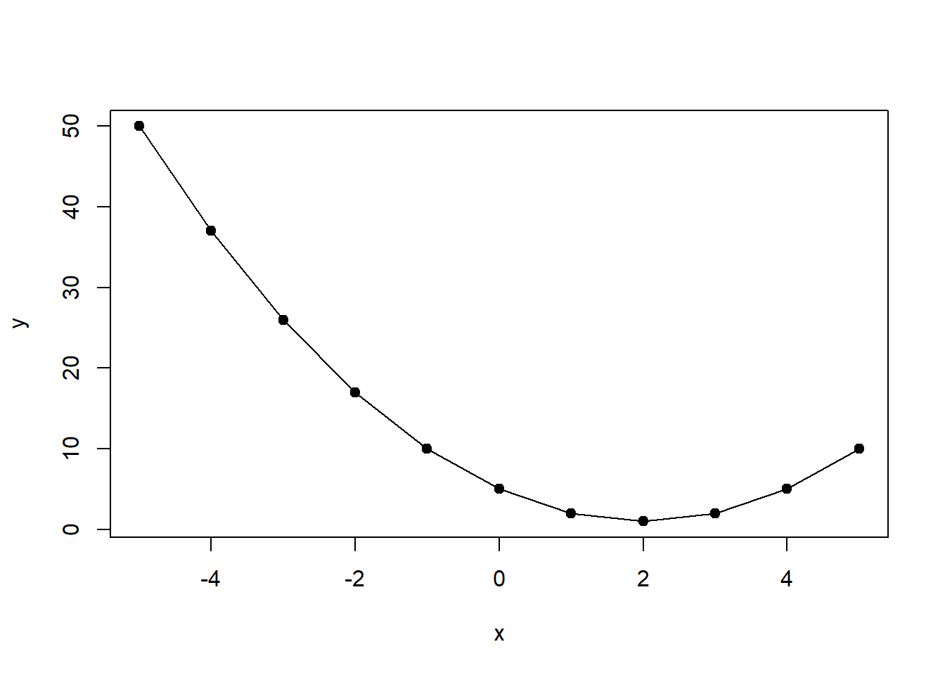
Once a critical point is identified, the next step is to determine whether that point is a minima or a maxima. The most straightforward way to do this is to identify the x,y coordinates and plot. This can be done in R, as we will show using the function y=f(x)=(x2−4x+5)y=f(x)=(x2−4x+5). The plot is shown in Figure \(\PageIndex{3}\).

x <- c(-5:5)
x

##  [1] -5 -4 -3 -2 -1  0  1  2  3  4  5

y <- x^2-4*x+5
y

##  [1] 50 37 26 17 10  5  2  1  2  5 10

plot(x,y, type="o", pch=19)

Figure \(\PageIndex{3}\): Identification of Critical Points

As can be seen, the critical point (2,1)(2,1) is a minima.

8.1.3 Partial Derivation

When an equation includes two variables, one can take a partial derivative with respect to only one variable, while the other variable is simply treated as a constant. This is particularly useful in our case because the function ∑ϵ2∑ϵ2 has two variables – ^αα^ and ^ββ^.

Let’s take an example. For the function y=f(x,z)=x3+4xz−5z2y=f(x,z)=x3+4xz−5z2, we first take the derivative of xx holding zz constant.

∂y∂x=∂f(x,z)∂x=3x2+4z∂y∂x=∂f(x,z)∂x=3x2+4z

Next we take the derivative of zz holding xx constant.

∂y∂z=∂f(x,z)∂z=4x−10z