13.5: Happiness and Well-Being

Researchers are interested in explaining differences in how happy people are based on how healthy people are. They gather data on each of these variables from 18 people and fit a linear regression model to explain the variance. We will follow the four-step hypothesis testing procedure to see if there is a relation between these variables that is statistically significant.

Step 1: State the Hypotheses

The null hypothesis in regression states that there is no relation between our variables. The alternative states that there is a relation, but because our research description did not explicitly state a direction of the relation, we will use a nondirectional hypothesis.

\[\begin{array}{c}{\text { Ho }_{0}: \text { There is no explanatory relation between health and happiness }} \\ {\qquad \mathrm{H}_{0}: \beta=0}\end{array} \nonumber \]

\[\begin{array}{c}{\text { H}_{ A } : \text { There is an explanatory relation between health and happiness } } \\ {\qquad \mathrm{H}_{\mathrm{A}}: \beta \neq 0}\end{array} \nonumber \]

Step 2: Find the Critical Value

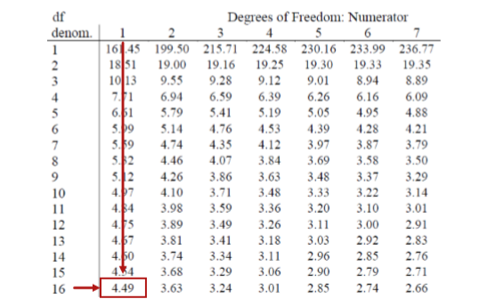
Because regression and ANOVA are the same analysis, our critical value for regression will come from the same place: the \(F\) distribution table, which uses two types of degrees of freedom. We saw above that the degrees of freedom for our numerator – the Model line – is always 1 in simple linear regression, and that the denominator degrees of freedom – from the Error line – is \(N – 2\). In this instance, we have 18 people so our degrees of freedom for the denominator is 16. Going to our \(F\) table, we find that the appropriate critical value for 1 and 16 degrees of freedom is \(F^* = 4.49\), shown below in Figure \(\PageIndex{1}\).

Figure \(\PageIndex{1}\): Critical value from F distribution table

Step 3: Calculate the Test Statistic

The process of calculating the test statistic for regression first involves computing the parameter estimates for the line of best fit. To do this, we first calculate the means, standard deviations, and sum of products for our \(X\) and \(Y\) variables, as shown below.

Table \(\PageIndex{1}\): Sum of Products table

\(X\)	\((X-\overline{X})\)	\((X-\overline{X})^2\)	\(Y\)	\((Y-\overline{Y})\)	\((Y-\overline{Y})^2\)	\((X-\overline{X})(Y-\overline{Y})\)
17.65	-2.13	4.53	10.36	-7.10	50.37	15.10
16.99	-2.79	7.80	16.38	-1.08	1.16	3.01
18.30	-1.48	2.18	15.23	-2.23	4.97	3.29
18.28	-1.50	2.25	14.26	-3.19	10.18	4.79
21.89	2.11	4.47	17.71	0.26	0.07	0.55
22.61	2.83	8.01	16.47	-0.98	0.97	-2.79
17.42	-2.36	5.57	16.89	-0.56	0.32	1.33
20.35	0.57	0.32	18.74	1.29	1.66	-0.09.73
18.89	-0.89	0.79	21.96	4.50	20.26	-4.00
18.63	-1.15	1.32	17.57	0.11	0.01	-0.13
19.67	-0.11	0.01	18.12	0.66	0.44	-0.08
18.39	-1.39	1.94	12.08	-5.37	28.87	7.48
22.48	2.71	7.32	17.11	-0.34	0.12	-0.93
23.25	3.47	12.07	21.66	4.21	17.73	14.63
19.91	0.13	0.02	17.86	0.40	0.16	0.05
18.21	-1.57	2.45	18.49	1.03	1.07	-1.62
23.65	3.87	14.99	22.13	4.67	21.82	18.08
19.45	-0.33	0.11	21.17	3.72	13.82	-1.22
356.02	0.00	76.14	314.18	0.00	173.99	58.29

From the raw data in our \(X\) and \(Y\) columns, we find that the means are \(\overline{\mathrm{X}}=19.78\) and \(\overline{\mathrm{Y}}=17.45\). The deviation scores for each variable sum to zero, so all is well there. The sums of squares for \(X\) and \(Y\) ultimately lead us to standard deviations of \(s_{X}=2.12\) and \(s_{Y}=3.20\). Finally, our sum of products is 58.29, which gives us a covariance of \(\operatorname{cov}_{X Y}=3.43\), so we know our relation will be positive. This is all the information we need for our equations for the line of best.

First, we must calculate the slope of the line:

\[\mathrm{b}=\dfrac{S P}{S S X}=\dfrac{58.29}{76.14}=0.77 \nonumber \]

This means that as \(X\) changes by 1 unit, \(Y\) will change by 0.77. In terms of our problem, as health increases by 1, happiness goes up by 0.77, which is a positive relation. Next, we use the slope, along with the means of each variable, to compute the intercept:

\[\begin{aligned} a &=\overline{Y}-b\: \overline{X} \\ a=& 17.45-0.77 * 19.78 \\ a=& 17.45-15.03=2.42 \end{aligned} \nonumber \]

For this particular problem (and most regressions), the intercept is not an important or interpretable value, so we will not read into it further. Now that we have all of our parameters estimated, we can give the full equation for our line of best fit:

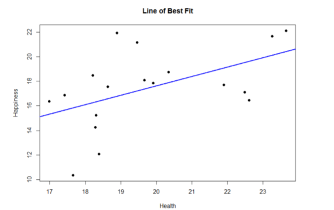
\[\widehat{\mathrm{Y}}=2.42+0.77 \mathrm{X} \nonumber \]

We can plot this relation in a scatterplot and overlay our line onto it, as shown in Figure \(\PageIndex{2}\).

Figure \(\PageIndex{2}\): Health and happiness data and line.

We can use the line equation to find predicted values for each observation and use them to calculate our sums of squares model and error, but this is tedious to do by hand, so we will let the computer software do the heavy lifting in that column of our ANOVA table:

Table \(\PageIndex{2}\): ANOVA Table

Source	\(SS\)	\(df\)	\(MS\)	\(F\)
Model	44.62
Error	129.37
Total

Now that we have these, we can fill in the rest of the ANOVA table. We already found our degrees of freedom in Step 2:

Table \(\PageIndex{3}\): ANOVA Table

Source	\(SS\)	\(df\)	\(MS\)	\(F\)
Model	44.62	1
Error	129.37	16
Total

Our total line is always the sum of the other two lines, giving us:

Table \(\PageIndex{4}\): ANOVA Table

Source	\(SS\)	\(df\)	\(MS\)	\(F\)
Model	44.62	1
Error	129.37	16
Total	173.99	17

Our mean squares column is only calculated for the model and error lines and is always our \(SS\) divided by our \(df\), which is:

Table \(\PageIndex{5}\): ANOVA Table

Source	\(SS\)	\(df\)	\(MS\)	\(F\)
Model	44.62	1	44.62
Error	129.37	16	8.09
Total	173.99	17

Finally, our \(F\) statistic is the ratio of the mean squares:

Table \(\PageIndex{6}\): ANOVA Table

Source	\(SS\)	\(df\)	\(MS\)	\(F\)
Model	44.62	1	44.62	5.52
Error	129.37	16	8.09
Total	173.99	17

This gives us an obtained \(F\) statistic of 5.52, which we will now use to test our hypothesis.

Step 4: Make the Decision

We now have everything we need to make our final decision. Our obtained test statistic was \(F = 5.52\) and our critical value was \(F^* = 4.49\). Since our obtained test statistic is greater than our critical value, we can reject the null hypothesis.

Reject \(H_0\). Based on our sample of 18 people, we can predict levels of happiness based on how healthy someone is, \(F(1,16) = 5.52, p < .05\).

Effect Size We know that, because we rejected the null hypothesis, we should calculate an effect size. In regression, our effect size is variance explained, just like it was in ANOVA. Instead of using \(η^2\) to represent this, we instead us \(R^2\), as we saw in correlation (yet more evidence that all of these are the same analysis). Variance explained is still the ratio of \(SS_M\) to \(SS_T\):

\[R^{2}=\dfrac{S S_{M}}{S S_{T}}=\dfrac{44.62}{173.99}=0.26 \nonumber \]

We are explaining 26% of the variance in happiness based on health, which is a large effect size (\(R^2\) uses the same effect size cutoffs as \(η^2\)).

Accuracy in Prediction

We found a large, statistically significant relation between our variables, which is what we hoped for. However, if we want to use our estimated line of best fit for future prediction, we will also want to know how precise or accurate our predicted values are. What we want to know is the average distance from our predictions to our actual observed values, or the average size of the residual (\(Y − \widehat {Y}\)). The average size of the residual is known by a specific name: the standard error of the estimate (\(S_{(Y-\widehat{Y})}\)), which is given by the formula

\[S_{(Y-\widehat{Y})}=\sqrt{\dfrac{\sum(Y-\widehat{Y})^{2}}{N-2}} \]

This formula is almost identical to our standard deviation formula, and it follows the same logic. We square our residuals, add them up, then divide by the degrees of freedom. Although this sounds like a long process, we already have the sum of the squared residuals in our ANOVA table! In fact, the value under the square root sign is just the \(SS_E\) divided by the \(df_E\), which we know is called the mean squared error, or \(MS_E\):

\[s_{(Y-\widehat{Y})}=\sqrt{\dfrac{\sum(Y-\widehat{Y})^{2}}{N-2}}=\sqrt{M S E} \]

For our example:

\[s_{(Y-\widehat{Y})}=\sqrt{\dfrac{129.37}{16}}=\sqrt{8.09}=2.84 \nonumber \]

So on average, our predictions are just under 3 points away from our actual values. There are no specific cutoffs or guidelines for how big our standard error of the estimate can or should be; it is highly dependent on both our sample size and the scale of our original \(Y\) variable, so expert judgment should be used. In this case, the estimate is not that far off and can be considered reasonably precise.