Estimation

CO-4: Distinguish among different measurement scales, choose the appropriate descriptive and inferential statistical methods based on these distinctions, and interpret the results.

CO-6: Apply basic concepts of probability, random variation, and commonly used statistical probability distributions.

Video

Video: Estimation (11:40)

Introduction

In our Introduction to Inference we defined point estimates and interval estimates.

• In point estimation, we estimate an unknown parameter using a single number that is calculated from the sample data.

• In interval estimation, we estimate an unknown parameter using an interval of values that is likely to contain the true value of that parameter (and state how confident we are that this interval indeed captures the true value of the parameter).

In this section, we will introduce the concept of a confidence interval and learn to calculate confidence intervals for population means and population proportions (when certain conditions are met).

In Unit 4B, we will see that confidence intervals are useful whenever we wish to use data to estimate an unknown population parameter, even when this parameter is estimated using multiple variables (such as our cases: CC, CQ, QQ).

For example, we can construct confidence intervals for the slope of a regression equation or the correlation coefficient. In doing so we are always using our data to provide an interval estimate for an unknown population parameter (the TRUE slope, or the TRUE correlation coefficient).

Point Estimation

Learning Objectives

LO 4.29: Determine and use the correct point estimates for specified population parameters.

Point estimation is the form of statistical inference in which, based on the sample data, we estimate the unknown parameter of interest using a single value (hence the name point estimation). As the following two examples illustrate, this form of inference is quite intuitive.

EXAMPLE:

Suppose that we are interested in studying the IQ levels of students at Smart University (SU). In particular (since IQ level is a quantitative variable), we are interested in estimating µ (mu), the mean IQ level of all the students at SU.

A random sample of 100 SU students was chosen, and their (sample) mean IQ level was found to be 115 (x-bar).

If we wanted to estimate µ (mu), the population mean IQ level, by a single number based on the sample, it would make intuitive sense to use the corresponding quantity in the sample, the sample mean which is 115. We say that 115 is the point estimate for µ (mu), and in general, we’ll always use the sample mean (x-bar) as the point estimator for µ (mu). (Note that when we talk about the specific value (115), we use the term estimate, and when we talk in general about the statistic x-bar, we use the term estimator. The following figure summarizes this example:

Here is another example.

EXAMPLE:

Suppose that we are interested in the opinions of U.S. adults regarding legalizing the use of marijuana. In particular, we are interested in the parameter p, the proportion of U.S. adults who believe marijuana should be legalized.

Suppose a poll of 1,000 U.S. adults finds that 560 of them believe marijuana should be legalized. If we wanted to estimate p, the population proportion, using a single number based on the sample, it would make intuitive sense to use the corresponding quantity in the sample, the sample proportion p-hat = 560/1000 = 0.56. We say in this case that 0.56 is the point estimate for p, and in general, we’ll always use p-hat as the point estimator for p. (Note, again, that when we talk about the specific value (0.56), we use the term estimate, and when we talk in general about the statistic p-hat, we use the term estimator. Here is a visual summary of this example:

Did I Get This?: Point Estimation

Desired Properties of Point Estimators

You may feel that since it is so intuitive, you could have figured out point estimation on your own, even without the benefit of an entire course in statistics. Certainly, our intuition tells us that the best estimator for the population mean (mu, µ) should be x-bar, and the best estimator for the population proportion p should be p-hat.

Probability theory does more than this; it actually gives an explanation (beyond intuition) why x-bar and p-hat are the good choices as point estimators for µ (mu) and p, respectively. In the Sampling Distributions section of the Probability unit, we learned about the sampling distribution of x-bar and found that as long as a sample is taken at random, the distribution of sample means is exactly centered at the value of population mean.

Our statistic, x-bar, is therefore said to be an unbiased estimator for µ (mu). Any particular sample mean might turn out to be less than the actual population mean, or it might turn out to be more. But in the long run, such sample means are “on target” in that they will not underestimate any more or less often than they overestimate.

Likewise, we learned that the sampling distribution of the sample proportion, p-hat, is centered at the population proportion p (as long as the sample is taken at random), thus making p-hat an unbiased estimator for p.

As stated in the introduction, probability theory plays an essential role as we establish results for statistical inference. Our assertion above that sample mean and sample proportion are unbiased estimators is the first such instance.

Importance of Sampling and Design

Notice how important the principles of sampling and design are for our above results: if the sample of U.S. adults in (example 2 on the previous page) was not random, but instead included predominantly college students, then 0.56 would be a biased estimate for p, the proportion of all U.S. adults who believe marijuana should be legalized.

If the survey design were flawed, such as loading the question with a reminder about the dangers of marijuana leading to hard drugs, or a reminder about the benefits of marijuana for cancer patients, then 0.56 would be biased on the low or high side, respectively.

Caution

Our point estimates are truly unbiased estimates for the population parameter only if the sample is random and the study design is not flawed.

Standard Error and Sample Size

Not only are the sample mean and sample proportion on target as long as the samples are random, but their precision improves as sample size increases.

Again, there are two “layers” here for explaining this.

Intuitively, larger sample sizes give us more information with which to pin down the true nature of the population. We can therefore expect the sample mean and sample proportion obtained from a larger sample to be closer to the population mean and proportion, respectively. In the extreme, when we sample the whole population (which is called a census), the sample mean and sample proportion will exactly coincide with the population mean and population proportion.There is another layer here that, again, comes from what we learned about the sampling distributions of the sample mean and the sample proportion. Let’s use the sample mean for the explanation.

Recall that the sampling distribution of the sample mean x-bar is, as we mentioned before, centered at the population mean µ (mu)and has a standard error (standard deviation of the statistic, x-bar) of

standard deviation of \(\dfrac{\sigma}{\sqrt{n}}\)

As a result, as the sample size n increases, the sampling distribution of x-bar gets less spread out. This means that values of x-bar that are based on a larger sample are more likely to be closer to µ (mu) (as the figure below illustrates):

Similarly, since the sampling distribution of p-hat is centered at p and has a

standard deviation of \(\sqrt{\dfrac{p(1-p)}{n}}\)

which decreases as the sample size gets larger, values of p-hat are more likely to be closer to p when the sample size is larger.

Another Point Estimator

Another example of a point estimator is using sample standard deviation,

\(s=\sqrt{\dfrac{\sum_{i=1}^{n}\left(x_{i}-\bar{x}\right)^{2}}{n-1}}\)

to estimate population standard deviation, σ (sigma).

In this course, we will not be concerned with estimating the population standard deviation for its own sake, but since we will often substitute the sample standard deviation (s) for σ (sigma) when standardizing the sample mean, it is worth pointing out that s is an unbiased estimator for σ (sigma).

If we had divided by n instead of n – 1 in our estimator for population standard deviation, then in the long run our sample variance would be guilty of a slight underestimation. Division by n – 1 accomplishes the goal of making this point estimator unbiased.

The reason that our formula for s, introduced in the Exploratory Data Analysis unit, involves division by n – 1 instead of by n is the fact that we wish to use unbiased estimators in practice.

Let’s Summarize

• We use p-hat (sample proportion) as a point estimator for p (population proportion). It is an unbiased estimator: its long-run distribution is centered at p as long as the sample is random.

• We use x-bar (sample mean) as a point estimator for µ (mu, population mean). It is an unbiased estimator: its long-run distribution is centered at µ (mu) as long as the sample is random.

• In both cases, the larger the sample size, the more precise the point estimator is. In other words, the larger the sample size, the more likely it is that the sample mean (proportion) is close to the unknown population mean (proportion).

Did I Get This?: Properties of Point Estimators

Interval Estimation

Point estimation is simple and intuitive, but also a bit problematic. Here is why:

When we estimate μ (mu) by the sample mean x-bar we are almost guaranteed to make some kind of error. Even though we know that the values of x-bar fall around μ (mu), it is very unlikely that the value of x-bar will fall exactly at μ (mu).

Given that such errors are a fact of life for point estimates (by the mere fact that we are basing our estimate on one sample that is a small fraction of the population), these estimates are in themselves of limited usefulness, unless we are able to quantify the extent of the estimation error. Interval estimation addresses this issue. The idea behind interval estimation is, therefore, to enhance the simple point estimates by supplying information about the size of the error attached.

In this introduction, we’ll provide examples that will give you a solid intuition about the basic idea behind interval estimation.

EXAMPLE:

Consider the example that we discussed in the point estimation section:

Suppose that we are interested in studying the IQ levels of students attending Smart University (SU). In particular (since IQ level is a quantitative variable), we are interested in estimating μ (mu), the mean IQ level of all the students in SU. A random sample of 100 SU students was chosen, and their (sample) mean IQ level was found to be 115 (x-bar).

In point estimation we used x-bar = 115 as the point estimate for μ (mu). However, we had no idea of what the estimation error involved in such an estimation might be. Interval estimation takes point estimation a step further and says something like:

“I am 95% confident that by using the point estimate x-bar = 115 to estimate μ (mu), I am off by no more than 3 IQ points. In other words, I am 95% confident that μ (mu) is within 3 of 115, or between 112 (115 – 3) and 118 (115 + 3).”

Yet another way to say the same thing is: I am 95% confident that μ (mu) is somewhere in (or covered by) the interval (112,118). (Comment: At this point you should not worry about, or try to figure out, how we got these numbers. We’ll do that later. All we want to do here is make sure you understand the idea.)

Note that while point estimation provided just one number as an estimate for μ (mu) of 115, interval estimation provides a whole interval of “plausible values” for μ (mu) (between 112 and 118), and also attaches the level of our confidence that this interval indeed includes the value of μ (mu) to our estimation (in our example, 95% confidence). The interval (112,118) is therefore called “a 95% confidence interval for μ (mu).”

Let’s look at another example:

EXAMPLE:

Let’s consider the second example from the point estimation section.

Suppose that we are interested in the opinions of U.S. adults regarding legalizing the use of marijuana. In particular, we are interested in the parameter p, the proportion of U.S. adults who believe marijuana should be legalized.

Suppose a poll of 1,000 U.S. adults finds that 560 of them believe marijuana should be legalized.

If we wanted to estimate p, the population proportion, by a single number based on the sample, it would make intuitive sense to use the corresponding quantity in the sample, the sample proportion p-hat = 560/1000=0.56.

Interval estimation would take this a step further and say something like:

“I am 90% confident that by using 0.56 to estimate the true population proportion, p, I am off by (or, I have an error of) no more than 0.03 (or 3 percentage points). In other words, I am 90% confident that the actual value of p is somewhere between 0.53 (0.56 – 0.03) and 0.59 (0.56 + 0.03).”

Yet another way of saying this is: “I am 90% confident that p is covered by the interval (0.53, 0.59).”

In this example, (0.53, 0.59) is a 90% confidence interval for p.

Let’s summarize

The two examples showed us that the idea behind interval estimation is, instead of providing just one number for estimating an unknown parameter of interest, to provide an interval of plausible values of the parameter plus a level of confidence that the value of the parameter is covered by this interval.

We are now going to go into more detail and learn how these confidence intervals are created and interpreted in context. As you’ll see, the ideas that were developed in the “Sampling Distributions” section of the Probability unit will, again, be very important. Recall that for point estimation, our understanding of sampling distributions leads to verification that our statistics are unbiased and gives us a precise formulas for the standard error of our statistics.

We’ll start by discussing confidence intervals for the population mean μ (mu), and later discuss confidence intervals for the population proportion p.

Population Means (Part 1)

CO-4: Distinguish among different measurement scales, choose the appropriate descriptive and inferential statistical methods based on these distinctions, and interpret the results.

Learning Objectives

LO 4.30: Interpret confidence intervals for population parameters in context.

Learning Objectives

LO 4.31: Find confidence intervals for the population mean using the normal distribution (Z) based confidence interval formula (when required conditions are met) and perform sample size calculations.

CO-6: Apply basic concepts of probability, random variation, and commonly used statistical probability distributions.

Learning Objectives

LO 6.24: Explain the connection between the sampling distribution of a statistic, and its properties as a point estimator.

Learning Objectives

LO 6.25: Explain what a confidence interval represents and determine how changes in sample size and confidence level affect the precision of the confidence interval.

Video

Video: Population Means – Part 1 (11:14)

As the introduction mentioned, we’ll start our discussion on interval estimation with interval estimation for the population mean μ (mu). We’ll start by showing how a 95% confidence interval is constructed, and later generalize to other levels of confidence. We’ll also discuss practical issues related to interval estimation.

Recall the IQ example:

EXAMPLE:

Suppose that we are interested in studying the IQ levels of students at Smart University (SU). In particular (since IQ level is a quantitative variable), we are interested in estimating μ (mu), the mean IQ level of all the students at SU.

We will assume that from past research on IQ scores in different universities, it is known that the IQ standard deviation in such populations is σ (sigma) = 15. In order to estimate μ (mu), a random sample of 100 SU students was chosen, and their (sample) mean IQ level is calculated (let’s assume, for now, that we have not yet found the sample mean).

We will now show the rationale behind constructing a 95% confidence interval for the population mean μ (mu).

• We learned in the “Sampling Distributions” section of probability that according to the central limit theorem, the sampling distribution of the sample mean x-bar is approximately normal with a mean of μ (mu) and standard deviation of σ/sqrt(n) = sigma/sqrt(n). In our example, then, (where σ (sigma) = 15 and n = 100), the possible values of x-bar, the sample mean IQ level of 100 randomly chosen students, is approximately normal, with mean μ (mu) and standard deviation 15/sqrt(100) = 1.5.
• Next, we recall and apply the Standard Deviation Rule for the normal distribution, and in particular its second part: There is a 95% chance that the sample mean we will find in our sample falls within 2 * 1.5 = 3 of μ (mu).

Obviously, if there is a certain distance between the sample mean and the population mean, we can describe that distance by starting at either value. So, if the sample mean (x-bar) falls within a certain distance of the population mean μ (mu), then the population mean μ (mu) falls within the same distance of the sample mean.

Therefore, the statement, “There is a 95% chance that the sample mean x-bar falls within 3 units of μ (mu)” can be rephrased as: “We are 95% confident that the population mean μ (mu) falls within 3 units of the x-bar we found in our sample.”

So, if we happen to get a sample mean of x-bar = 115, then we are 95% confident that μ (mu) falls within 3 units of 115, or in other words that μ (mu) is covered by the interval (115 – 3, 115 + 3) = (112,118).

(On later pages, we will use similar reasoning to develop a general formula for a confidence interval.)

Comment:

• Note that the first phrasing is about x-bar, which is a random variable; that’s why it makes sense to use probability language. But the second phrasing is about μ (mu), which is a parameter, and thus is a “fixed” value that does not change, and that’s why we should not use probability language to discuss it. In these problems, it is our x-bar that will change when we repeat the process, not μ (mu). This point will become clearer after you do the activities which follow.

The General Case

Let’s generalize the IQ example. Suppose that we are interested in estimating the unknown population mean (μ, mu) based on a random sample of size n. Further, we assume that the population standard deviation (σ, sigma) is known.

Caution

Note: The assumption that the population standard deviation is known is not usually realistic, however, we make it here to be able to introduce the concepts in the simplest case. Later, we will discuss the changes which need to be made when we do not know the population standard deviation.

The values of x-bar follow a normal distribution with (unknown) mean μ (mu) and standard deviation σ/sqrt(n)=sigma/sqrt(n) (known, since both σ, sigma, and n are known). In the standard deviation rule, we stated that approximately 95% of values fall within 2 standard deviations of μ (mu). From now on, we will be a little more precise and use the standard normal table to find the exact value for 95%.

Our picture is as follows:

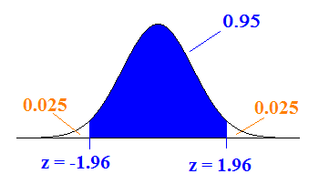
Try using the applet in the post for Learn by Doing – Normal Random Variables to find the cutoff illustrated above.

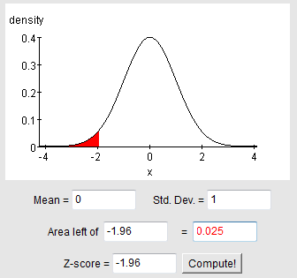
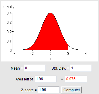
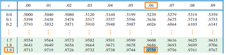
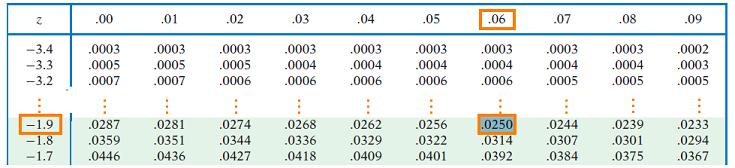
We can also verify the z-score using a calculator or table by finding the z-score with the area of 0.025 to the left (which would give us -1.96) or with the area to the left of 0.975 = 0.95 + 0.025 (which would give us +1.96).

Thus, there is a 95% chance that our sample mean x-bar will fall within 1.96*σ/sqrt(n) = 1.96*sigma/sqrt(n) of μ (mu).

Which means we are 95% confident that μ (mu) falls within 1.96*σ/sqrt(n) = 1.96*sigma/sqrt(n) of our sample mean x-bar.

Here, then, is the general result:

Suppose a random sample of size n is taken from a normal population of values for a quantitative variable whose mean (μ, mu) is unknown, when the standard deviation (σ, sigma) is given.

A 95% confidence interval (CI) for μ (mu) is:

\(\bar{x} \pm 1.96 * \dfrac{\sigma}{\sqrt{n}}\)

Comment:

• Note that for now we require the population standard deviation (σ, sigma) to be known. Practically, σ (sigma) is rarely known, but for some cases, especially when a lot of research has been done on the quantitative variable whose mean we are estimating (such as IQ, height, weight, scores on standardized tests), it is reasonable to assume that σ (sigma) is known. Eventually, we will see how to proceed when σ (sigma) is unknown, and must be estimated with sample standard deviation (s).

Let’s look at another example.

EXAMPLE:

An educational researcher was interested in estimating μ (mu), the mean score on the math part of the SAT (SAT-M) of all community college students in his state. To this end, the researcher has chosen a random sample of 650 community college students from his state, and found that their average SAT-M score is 475. Based on a large body of research that was done on the SAT, it is known that the scores roughly follow a normal distribution with the standard deviation σ (sigma) =100.

Here is a visual representation of this story, which summarizes the information provided:

Based on this information, let’s estimate μ (mu) with a 95% confidence interval.

Using the formula we developed earlier

\(\bar{x} \pm 1.96 * \dfrac{\simga}{\sqrt{n}}\)

the 95% confidence interval for μ (mu) is:

\begin{aligned}
475 \pm 1.96 * \frac{100}{\sqrt{650}} &=\left(475-1.96 * \frac{100}{\sqrt{650}}, 475+1.96 * \frac{100}{\sqrt{650}}\right) \\
&=(475-7.7,475+7.7) \\
&=(467.3,482.7)
\end{aligned}

We will usually provide information on how to round your final answer. In this case, one decimal place is enough precision for this scenario. You could also round to the nearest whole number without much loss of information here.

We are not done yet. An equally important part is to interpret what this means in the context of the problem.

We are 95% confident that the mean SAT-M score of all community college students in the researcher’s state is covered by the interval (467.3, 482.7). Note that the confidence interval was obtained by taking 475 ± 7.7. This means that we are 95% confident that by using the sample mean (x-bar = 475) to estimate μ (mu), our error is no more than 7.7 points.

Learn by Doing: Confidence Intervals: Means #1

You just gained practice computing and interpreting a confidence interval for a population mean. Note that the way a confidence interval is used is that we hope the interval contains the population mean μ (mu). This is why we call it an “interval for the population mean.”

The following activity is designed to help give you a better understanding of the underlying reasoning behind the interpretation of confidence intervals. In particular, you will gain a deeper understanding of why we say that we are “95% confident that the population mean is covered by the interval.”

Learn by Doing: Connection between Confidence Intervals and Sampling Distributions with Video (1:18)

We just saw that one interpretation of a 95% confidence interval is that we are 95% confident that the population mean (μ, mu) is contained in the interval. Another useful interpretation in practice is that, given the data, the confidence interval represents the set of plausible values for the population mean μ (mu).

EXAMPLE:

As an illustration, let’s return to the example of mean SAT-Math score of community college students. Recall that we had constructed the confidence interval (467.3, 482.7) for the unknown mean SAT-M score for all community college students.

Here is a way that we can use the confidence interval:

Do the results of this study provide evidence that μ (mu), the mean SAT-M score of community college students, is lower than the mean SAT-M score in the general population of college students in that state (which is 480)?

The 95% confidence interval for μ (mu) was found to be (467.3, 482.7). Note that 480, the mean SAT-M score in the general population of college students in that state, falls inside the interval, which means that it is one of the plausible values for μ (mu).

This means that μ (mu) could be 480 (or even higher, up to 483), and therefore we cannot conclude that the mean SAT-M score among community college students in the state is lower than the mean in the general population of college students in that state. (Note that the fact that most of the plausible values for μ (mu) fall below 480 is not a consideration here.)

\(\bar{x} \pm 1.96 * \dfrac{\sigma}{\sqrt{n}}\)

the 95% confidence interval for μ (mu) is:

\begin{aligned}
475 \pm 1.96 * \frac{100}{\sqrt{650}} &=\left(475-1.96 * \frac{100}{\sqrt{650}}, 475+1.96 * \frac{100}{\sqrt{650}}\right) \\
&=(475-7.7,475+7.7) \\
&=(467.3,482.7)
\end{aligned}

We will usually provide information on how to round your final answer. In this case, one decimal place is enough precision for this scenario. You could also round to the nearest whole number without much loss of information here.

We are not done yet. An equally important part is to interpret what this means in the context of the problem.

We are 95% confident that the mean SAT-M score of all community college students in the researcher’s state is covered by the interval (467.3, 482.7). Note that the confidence interval was obtained by taking 475 ± 7.7. This means that we are 95% confident that by using the sample mean (x-bar = 475) to estimate μ (mu), our error is no more than 7.7 points.

Population Means (Part 2)

CO-4: Distinguish among different measurement scales, choose the appropriate descriptive and inferential statistical methods based on these distinctions, and interpret the results.

Learning Objectives

LO 4.30: Interpret confidence intervals for population parameters in context.

Learning Objectives

LO 4.31: Find confidence intervals for the population mean using the normal distribution (Z) based confidence interval formula (when required conditions are met) and perform sample size calculations.

CO-6: Apply basic concepts of probability, random variation, and commonly used statistical probability distributions.

Learning Objectives

LO 6.24: Explain the connection between the sampling distribution of a statistic, and its properties as a point estimator.

Learning Objectives

LO 6.25: Explain what a confidence interval represents and determine how changes in sample size and confidence level affect the precision of the confidence interval.

Video

Video: Population Means – Part 2 (4:04)

Other Levels of Confidence

95% is the most commonly used level of confidence. However, we may wish to increase our level of confidence and produce an interval that’s almost certain to contain μ (mu). Specifically, we may want to report an interval for which we are 99% confident that it contains the unknown population mean, rather than only 95%.

Using the same reasoning as in the last comment, in order to create a 99% confidence interval for μ (mu), we should ask: There is a probability of 0.99 that any normal random variable takes values within how many standard deviations of its mean? The precise answer is 2.576, and therefore, a 99% confidence interval for μ (mu) is:

\(\bar{x} \pm 2.576 * \dfrac{\sigma}{\sqrt{n}}\)

Another commonly used level of confidence is a 90% level of confidence. Since there is a probability of 0.90 that any normal random variable takes values within 1.645 standard deviations of its mean, the 90% confidence interval for μ (mu) is:

\(\bar{x} \pm 1.645 * \dfrac{\sigma}{\sqrt{n}}\)

EXAMPLE:

Let’s go back to our first example, the IQ example:

The IQ level of students at a particular university has an unknown mean (μ, mu) and known standard deviation σ (sigma) =15. A simple random sample of 100 students is found to have a sample mean IQ of 115 (x-bar). Estimate μ (mu) with a 90%, 95%, and 99% confidence interval.

A 90% confidence interval for μ (mu) is:

\(\bar{x} \pm 1.645 \dfrac{\sigma}{\sqrt{n}} = 115 \pm 1.645(\dfrac{15}{\sqrt{100}}) = 115 \pm 2.5 = (112.5, 117.5)\).

A 95% confidence interval for μ (mu) is:

\(\bar{x} \pm 1.96 \dfrac{\sigma}{\sqrt{n}} = 115 \pm 1.96 (\dfrac{15}{\sqrt{100}}) = 115 \pm 2.9 = (112.1, 117.9)\).

A 99% confidence interval for μ (mu) is:

\(\bar{x} \pm 2.576 \dfrac{\sigma}{\sqrt{n}} = 115 \pm 2.576 (\dfrac{15}{\sqrt{100}} = 115 \pm 4.0 = (111,119)\).

The purpose of this next activity is to give you guided practice at calculating and interpreting confidence intervals, and drawing conclusions from them.

Did I Get This?: Confidence Intervals: Means #1

Note from the previous example and the previous “Did I Get This?” activity, that the more confidence I require, the wider the confidence interval for μ (mu). The 99% confidence interval is wider than the 95% confidence interval, which is wider than the 90% confidence interval.

This is not very surprising, given that in the 99% interval we multiply the standard deviation of the statistic by 2.576, in the 95% by 2, and in the 90% only by 1.645. Beyond this numerical explanation, there is a very clear intuitive explanation and an important implication of this result.

Let’s start with the intuitive explanation. The more certain I want to be that the interval contains the value of μ (mu), the more plausible values the interval needs to include in order to account for that extra certainty. I am 95% certain that the value of μ (mu) is one of the values in the interval (112.1, 117.9). In order to be 99% certain that one of the values in the interval is the value of μ (mu), I need to include more values, and thus provide a wider confidence interval.

Learn by Doing: Visualizing the Relationship between Confidence and Width

In our example, the wider 99% confidence interval (111, 119) gives us a less precise estimation about the value of μ (mu) than the narrower 90% confidence interval (112.5, 117.5), because the smaller interval ‘narrows-in’ on the plausible values of μ (mu).

The important practical implication here is that researchers must decide whether they prefer to state their results with a higher level of confidence or produce a more precise interval. In other words,

Caution

There is a trade-off between the level of confidence and the precision with which the parameter is estimated.

The price we have to pay for a higher level of confidence is that the unknown population mean will be estimated with less precision (i.e., with a wider confidence interval). If we would like to estimate μ (mu) with more precision (i.e. a narrower confidence interval), we will need to sacrifice and report an interval with a lower level of confidence.

Did I Get This?: Confidence Intervals: Means #2

So far we’ve developed the confidence interval for the population mean “from scratch” based on results from probability, and discussed the trade-off between the level of confidence and the precision of the interval. The price you pay for a higher level of confidence is a lower level of precision of the interval (i.e., a wider interval).

Is there a way to bypass this trade-off? In other words, is there a way to increase the precision of the interval (i.e., make it narrower) without compromising on the level of confidence? We will answer this question shortly, but first we’ll need to get a deeper understanding of the different components of the confidence interval and its structure.

Understanding the General Structure of Confidence Intervals

We explored the confidence interval for μ (mu) for different levels of confidence, and found that in general, it has the following form:

\(\bar{x} \pm z* \dot \dfrac{\sigma}{\sqrt{n}}\)

where z* is a general notation for the multiplier that depends on the level of confidence. As we discussed before:

• For a 90% level of confidence, z* = 1.645

• For a 95% level of confidence, z* = 1.96

• For a 99% level of confidence, z* = 2.576

To start our discussion about the structure of the confidence interval, let’s denote

\(m = z* \dot \dfrac{\sigma}{\sqrt{n}}\)

The confidence interval, then, has the form:

\(\bar{x} \pm m\)

To summarize, we have

X-bar is the sample mean, the point estimator for the unknown population mean (μ, mu).

m is called the margin of error, since it represents the maximum estimation error for a given level of confidence.

For example, for a 95% confidence interval, we are 95% confident that our estimate will not depart from the true population mean by more than m, the margin of error and m is further made up of the product of two components:

Here is a summary of the different components of the confidence interval and its structure:

This structure: estimate ± margin of error, where the margin of error is further composed of the product of a confidence multiplier and the standard deviation of the statistic (or, as we’ll see, the standard error) is the general structure of all confidence intervals that we will encounter in this course.

Obviously, even though each confidence interval has the same components, the formula for these components is different from confidence interval to confidence interval, depending on what unknown parameter the confidence interval aims to estimate.

Since the structure of the confidence interval is such that it has a margin of error on either side of the estimate, it is centered at the estimate (in our current case, x-bar), and its width (or length) is exactly twice the margin of error:

The margin of error, m, is therefore “in charge” of the width (or precision) of the confidence interval, and the estimate is in charge of its location (and has no effect on the width).

Did I Get This?: Margin of Error

Let us now go back to the confidence interval for the mean, and more specifically, to the question that we posed at the beginning of the previous page:

Is there a way to increase the precision of the confidence interval (i.e., make it narrower) without compromising on the level of confidence?

Since the width of the confidence interval is a function of its margin of error, let’s look closely at the margin of error of the confidence interval for the mean and see how it can be reduced:

\(m = z* \dot \dfrac{\sigma}{\sqrt{n}}\)

Since z* controls the level of confidence, we can rephrase our question above in the following way:

Is there a way to reduce this margin of error other than by reducing z*?

If you look closely at the margin of error, you’ll see that the answer is yes. We can do that by increasing the sample size n (since it appears in the denominator).

Many Students Wonder: Confidence Intervals (Population Mean)

Question: Isn’t it true that another way to reduce the margin of error (for a fixed z*) is to reduce σ (sigma)?

Answer: While it is true that strictly mathematically speaking the smaller the value of σ (sigma), the smaller the margin of error, practically speaking we have absolutely no control over the value of σ (sigma) (i.e., we cannot make it larger or smaller). σ (sigma) is the population standard deviation; it is a fixed value (which here we assume is known) that has an effect on the width of the confidence interval (since it appears in the margin of error), but is definitely not a value we can change.

Let’s look at an example first and then explain why increasing the sample size is a way to increase the precision of the confidence interval without compromising on the level of confidence.

EXAMPLE:

Recall the IQ example:

The IQ level of students at a particular university has an unknown mean (μ, mu) and a known standard deviation of σ (sigma) =15. A simple random sample of 100 students is found to have the sample mean IQ of 115 (x-bar).

For simplicity, in this question, we will round z* = 1.96 to 2. You should use z* = 1.96 in all problems unless you are specifically instructed to do otherwise.

A 95% confidence interval for μ (mu) in this case is:

\(\bar{x} \pm 2 \dfrac{\sigma}{\sqrt{n}}=115 \pm 2\left(\dfrac{15}{\sqrt{100}}\right)=115 \pm 3.0=(112,118)\)

Note that the margin of error is m = 3, and therefore the width of the confidence interval is 6.

Now, what if we change the problem slightly by increasing the sample size, and assume that it was 400 instead of 100?

In this case, a 95% confidence interval for μ (mu) is:

\(\bar{x} \pm 2 \dfrac{\sigma}{\sqrt{n}}=115 \pm 2\left(\dfrac{15}{\sqrt{400}}\right)=115 \pm 1.5=(113.5,116.5)\)

The margin of error here is only m = 1.5, and thus the width is only 3.

Note that for the same level of confidence (95%) we now have a narrower, and thus more precise, confidence interval.

Let’s try to understand why is it that a larger sample size will reduce the margin of error for a fixed level of confidence. There are three ways to explain this: mathematically, using probability theory, and intuitively.

We’ve already alluded to the mathematical explanation; the margin of error is

\(m = z* \dot \dfrac{\sigma}{\sqrt{n}}\)

and since n, the sample size, appears in the denominator, increasing n will reduce the margin of error.

As we saw in our discussion about point estimates, probability theory tells us that:

This explains why with a larger sample size the margin of error (which represents how far apart we believe x-bar might be from μ (mu) for a given level of confidence) is smaller.

On an intuitive level, if our estimate x-bar is based on a larger sample (i.e., a larger fraction of the population), we have more faith in it, or it is more reliable, and therefore we need to account for less error around it.

Comment:

• While it is true that for a given level of confidence, increasing the sample size increases the precision of our interval estimation, in practice, increasing the sample size is not always possible.
  • Consider a study in which there is a non-negligible cost involved for collecting data from each participant (an expensive medical procedure, for example). If the study has some budgetary constraints, which is usually the case, increasing the sample size from 100 to 400 is just not possible in terms of cost-effectiveness.
  • Another instance in which increasing the sample size is impossible is when a larger sample is simply not available, even if we had the money to afford it. For example, consider a study on the effectiveness of a drug on curing a very rare disease among children. Since the disease is rare, there are a limited number of children who could be participants.
• This is the reality of statistics. Sometimes theory collides with reality, and you simply do the best you can.

Did I Get This?: Sample Size and Confidence

Population Means (Part 3)

CO-4: Distinguish among different measurement scales, choose the appropriate descriptive and inferential statistical methods based on these distinctions, and interpret the results.

Learning Objectives

LO 4.30: Interpret confidence intervals for population parameters in context.

Learning Objectives

LO 4.31: Find confidence intervals for the population mean using the normal distribution (Z) based confidence interval formula (when required conditions are met) and perform sample size calculations.

CO-6: Apply basic concepts of probability, random variation, and commonly used statistical probability distributions.

Learning Objectives

LO 6.24: Explain the connection between the sampling distribution of a statistic, and its properties as a point estimator.

Learning Objectives

LO 6.25: Explain what a confidence interval represents and determine how changes in sample size and confidence level affect the precision of the confidence interval.

Video

Video: Population Means – Part 3 (6:02)

Sample Size Calculations

As we just learned, for a given level of confidence, the sample size determines the size of the margin of error and thus the width, or precision, of our interval estimation. This process can be reversed.

In situations where a researcher has some flexibility as to the sample size, the researcher can calculate in advance what the sample size is that he/she needs in order to be able to report a confidence interval with a certain level of confidence and a certain margin of error. Let’s look at an example.

EXAMPLE:

Recall the example about the SAT-M scores of community college students.

An educational researcher is interested in estimating μ (mu), the mean score on the math part of the SAT (SAT-M) of all community college students in his state. To this end, the researcher has chosen a random sample of 650 community college students from his state, and found that their average SAT-M score is 475. Based on a large body of research that was done on the SAT, it is known that the scores roughly follow a normal distribution, with the standard deviation σ (sigma) =100.

The 95% confidence interval for μ (mu) is

\begin{aligned}
475 \pm 1.96 * \frac{100}{\sqrt{650}} &=\left(475-1.96 * \frac{100}{\sqrt{650}}, 475+1.96 * \frac{100}{\sqrt{650}}\right) \\
&=(475-7.7,475+7.7) \\
&=(467.3,482.7)
\end{aligned}

which is roughly 475 ± 8, or (467, 483). For a sample size of n = 650, our margin of error is 8.

Now, let’s think about this problem in a slightly different way:

An educational researcher is interested in estimating μ (mu), the mean score on the math part of the SAT (SAT-M) of all community college students in his state with a margin of error of (only) 5, at the 95% confidence level. What is the sample size needed to achieve this? σ (sigma), of course, is still assumed to be 100.

To solve this, we set:

\(m=2 \cdot \frac{100}{\sqrt{n}}=5 \quad \text { so } \quad \sqrt{n}=\frac{2(100)}{5} \quad \text { and } \quad n=\left(\frac{2(100)}{5}\right)^{2}=1600\)

So, for a sample size of 1,600 community college students, the researcher will be able to estimate μ (mu) with a margin of error of 5, at the 95% level. In this example, we can also imagine that the researcher has some flexibility in choosing the sample size, since there is a minimal cost (if any) involved in recording students’ SAT-M scores, and there are many more than 1,600 community college students in each state.

Rather than take the same steps to isolate n every time we solve such a problem, we may obtain a general expression for the required n for a desired margin of error m and a certain level of confidence.

Since

\(m = z* \dot \dfrac{\sigma}{\sqrt{n}}\)

is the formula to determine m for a given n, we can use simple algebra to express n in terms of m (multiply both sides by the square root of n, divide both sides by m, and square both sides) to get

\(n = (\dfrac{z* \sigma}{m})^2\)

Comment:

• Clearly, the sample size n must be an integer.
• In the previous example we got n = 1,600, but in other situations, the calculation may give us a non-integer result.
• In these cases, we should always round up to the next highest integer.
• Using this “conservative approach,” we’ll achieve an interval at least as narrow as the one desired.

EXAMPLE:

IQ scores are known to vary normally with a standard deviation of 15. How many students should be sampled if we want to estimate the population mean IQ at 99% confidence with a margin of error equal to 2?

\(n=\left(\dfrac{z^{*} \sigma}{m}\right)^{2}=\left(\dfrac{2.576(15)}{2}\right)^{2}=373.26\)

Round up to be safe, and take a sample of 374 students.

The purpose of the next activity is to give you guided practice in sample size calculations for obtaining confidence intervals with a desired margin of error, at a certain confidence level. Consider the example from the previous Learn By Doing activity:

Learn by Doing: Sample Size

Comment:

• In the preceding activity, you saw that in order to calculate the sample size when planning a study, you needed to know the population standard deviation, sigma (σ). In practice, sigma is usually not known, because it is a parameter. (The rare exceptions are certain variables like IQ score or standardized tests that might be constructed to have a particular known sigma.)

Therefore, when researchers wish to compute the required sample size in preparation for a study, they use an estimate of sigma. Usually, sigma is estimated based on the standard deviation obtained in prior studies.

However, in some cases, there might not be any prior studies on the topic. In such instances, a researcher still needs to get a rough estimate of the standard deviation of the (yet-to-be-measured) variable, in order to determine the required sample size for the study. One way to get such a rough estimate is with the “range rule of thumb.” We will not cover this topic in depth but mention here that a very rough estimate of the standard deviation of a population is the range/4.

There are a few more things we need to discuss:

• Is it always OK to use the confidence interval we developed for μ (mu) when σ (sigma) is known?

• What if σ (sigma) is unknown?

• How can we use statistical software to calculate confidence intervals for us?

When is it safe to use the confidence interval we developed?

One of the most important things to learn with any inference method is the conditions under which it is safe to use it. It is very tempting to apply a certain method, but if the conditions under which this method was developed are not met, then using this method will lead to unreliable results, which can then lead to wrong and/or misleading conclusions. As you’ll see throughout this section, we will always discuss the conditions under which each method can be safely used.

In particular, the confidence interval for μ (mu), when σ (sigma) is known:

\(\bar{x} \pm z* \dot \dfrac{\sigma}{\sqrt{n}}\)

was developed assuming that the sampling distribution of x-bar is normal; in other words, that the Central Limit Theorem applies. In particular, this allowed us to determine the values of z*, the confidence multiplier, for different levels of confidence.

First, the sample must be random. Assuming that the sample is random, recall from the Probability unit that the Central Limit Theorem works when the sample size is large (a common rule of thumb for “large” is n > 30), or, for smaller sample sizes, if it is known that the quantitative variable of interest is distributed normally in the population. The only situation when we cannot use the confidence interval, then, is when the sample size is small and the variable of interest is not known to have a normal distribution. In that case, other methods, called non-parametric methods, which are beyond the scope of this course, need to be used. This can be summarized in the following table:

Did I Get This?: When to Use Z-Interval (Means)

In the following activity, you have to opportunity to use software to summarize the raw data provided.

Did I Get This?: Confidence Intervals: Means #3

What if σ (sigma) is unknown?

As we discussed earlier, when variables have been well-researched in different populations it is reasonable to assume that the population standard deviation (σ, sigma) is known. However, this is rarely the case. What if σ (sigma) is unknown?

Well, there is some good news and some bad news.

The good news is that we can easily replace the population standard deviation, σ (sigma), with the sample standard deviation, s.

The bad news is that once σ (sigma) has been replaced by s, we lose the Central Limit Theorem, together with the normality of x-bar, and therefore the confidence multipliers z* for the different levels of confidence (1.645, 1.96, 2.576) are (generally) not correct any more. The new multipliers come from a different distribution called the “t distribution” and are therefore denoted by t* (instead of z*). We will discuss the t distribution in more detail when we talk about hypothesis testing.

The confidence interval for the population mean (μ, mu) when (σ, sigma) is unknown is therefore:

\(\bar{x} \pm t^{*} * \dfrac{s}{\sqrt{n}}\)

(Note that this interval is very similar to the one when σ (sigma) is known, with the obvious changes: s replaces σ (sigma), and t* replaces z* as discussed above.)

There is an important difference between the confidence multipliers we have used so far (z*) and those needed for the case when σ (sigma) is unknown (t*). Unlike the confidence multipliers we have used so far (z*), which depend only on the level of confidence, the new multipliers (t*) have the added complexity that they depend on both the level of confidence and on the sample size (for example: the t* used in a 95% confidence when n = 10 is different from the t* used when n = 40). Due to this added complexity in determining the appropriate t*, we will rely heavily on software in this case.

Comments:

• Since it is quite rare that σ (sigma) is known, this interval (sometimes called a “one-sample t confidence interval”) is more commonly used as the confidence interval for estimating μ (mu). (Nevertheless, we could not have presented it without our extended discussion up to this point, which also provided you with a solid understanding of confidence intervals.)

• The quantity s/sqrt(n) is called the estimated standard error of x-bar. The Central Limit Theorem tells us that σ/sqrt(n) = sigma/sqrt(n) is the standard deviation of x-bar (and this is the quantity used in confidence interval when σ (sigma) is known). In general, the standard error is the standard deviation of the sampling distribution of a statistic. When we substitute s for σ (sigma) we are estimating the true standard error. You may see the term “standard error” used for both the true standard error and the estimated standard error depending on the author and audience. What is important to understand about the standard error is that it measures the variation of a statistic calculated from a sample of a specified sample size (not the variation of the original population).

• As before, to safely use this confidence interval (one-sample t confidence interval), the sample must be random, and the only case when this interval cannot be used is when the sample size is small and the variable is not known to vary normally.

Final Comment:

• It turns out that for large values of n, the t* multipliers are not that different from the z* multipliers, and therefore using the interval formula:

\(\bar{x} \pm z* \ast \dfrac{s}{\sqrt{n}}\)

for μ (mu) when σ (sigma) is unknown provides a pretty good approximation.

Population Means (Summary)

Let’s summarize

• When the population is normal and/or the sample is large, a confidence interval for unknown population mean μ (mu) when σ (sigma) is known is:

\(\bar{x} \pm z* \dot \dfrac{\sigma}{\sqrt{n}}\)

where z* is 1.645 for 90% confidence, 1.96 for 95% confidence, and 2.576 for 99% confidence.

• There is a trade-off between the level of confidence and the precision of the interval estimation. For a given sample size, the price we have to pay for more precision is sacrificing level of confidence.

• The general form of confidence intervals is an estimate +/- the margin of error (m). In this case, the estimate = x-bar and

\(m = z* \dot \dfrac{\sigma}{\sqrt{n}}\)

The confidence interval is therefore centered at the estimate and its width is exactly 2m.

• For a given level of confidence, the width of the interval depends on the sample size. We can therefore do a sample size calculation to figure out what sample size is needed in order to get a confidence interval with a desired margin of error m, and a certain level of confidence (assuming we have some flexibility with the sample size). To do the sample size calculation we use:

\(n =( \dfrac{z* \sigma}{m})^2\)

(and round up to the next integer). We estimate σ (sigma) when necessary.

• When σ (sigma) is unknown, we use the sample standard deviation, s, instead, but as a result we also need to use a different set of confidence multipliers (t*) associated with the t distribution. We will use software to calculate intervals in this case, however, the formula for confidence interval in this case is

\(\bar{x} \pm t* \ast \dfrac{s}{\sqrt{n}}\)

• These new multipliers have the added complexity that they depend not only on the level of confidence, but also on the sample size. Software is therefore very useful for calculating confidence intervals in this case.

• For large values of n, the t* multipliers are not that different from the z* multipliers, and therefore using the interval formula:

\(\bar{x} \pm z* \ast \dfrac{s}{\sqrt{n}}\)

for μ (mu) when σ (sigma) is unknown provides a pretty good approximation.

Population Proportions

CO-4: Distinguish among different measurement scales, choose the appropriate descriptive and inferential statistical methods based on these distinctions, and interpret the results.

Learning Objectives

LO 4.30: Interpret confidence intervals for population parameters in context.

Learning Objectives

LO 4.32: Find confidence intervals for the population proportion using the formula (when required conditions are met) and perform sample size calculations.

CO-6: Apply basic concepts of probability, random variation, and commonly used statistical probability distributions.

Learning Objectives

LO 6.24: Explain the connection between the sampling distribution of a statistic, and its properties as a point estimator.

Learning Objectives

LO 6.25: Explain what a confidence interval represents and determine how changes in sample size and confidence level affect the precision of the confidence interval.

Video

Video: Population Proportions (4:13)

Confidence Intervals

As we mentioned in the introduction to Unit 4A, when the variable that we’re interested in studying in the population is categorical, the parameter we are trying to infer about is the population proportion (p) associated with that variable. We also learned that the point estimator for the population proportion p is the sample proportion p-hat.

To refresh your memory, here is a picture that summarizes an example we looked at.

We are now moving on to interval estimation of p. In other words, we would like to develop a set of intervals that, with different levels of confidence, will capture the value of p. We’ve actually done all the groundwork and discussed all the big ideas of interval estimation when we talked about interval estimation for μ (mu), so we’ll be able to go through it much faster. Let’s begin.

Recall that the general form of any confidence interval for an unknown parameter is:

estimate ± margin of error

Since the unknown parameter here is the population proportion p, the point estimator (as I reminded you above) is the sample proportion p-hat. The confidence interval for p, therefore, has the form:

(Recall that m is the notation for the margin of error.) The margin of error (m) gives us the maximum estimation error with a certain confidence. In this case it tells us that p-hat is different from p (the parameter it estimates) by no more than m units.

From our previous discussion on confidence intervals, we also know that the margin of error is the product of two components:

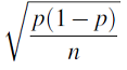
To figure out what these two components are, we need to go back to a result we obtained in the Sampling Distributions section of the Probability unit about the sampling distribution of p-hat. We found that under certain conditions (which we’ll come back to later), p-hat has a normal distribution with mean p, and a

This result makes things very simple for us, because it reveals what the two components are that the margin of error is made of:

• Since, like the sampling distribution of x-bar, the sampling distribution of p-hat is normal, the confidence multipliers that we’ll use in the confidence interval for p will be the same z* multipliers we use for the confidence interval for μ (mu) when σ (sigma) is known (using exactly the same reasoning and the same probability results). The multipliers we’ll use, then, are: 1.645, 1.96, and 2.576 at the 90%, 95% and 99% confidence levels, respectively.

• The standard deviation of our estimator p-hat is

Putting it all together, we find that the confidence interval for p should be:

We just have to solve one practical problem and we’re done. We’re trying to estimate the unknown population proportion p, so having it appear in the confidence interval doesn’t make any sense. To overcome this problem, we’ll do the obvious thing …

We’ll replace p with its sample counterpart, p-hat, and work with the estimated standard error of p-hat

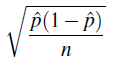
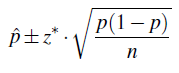
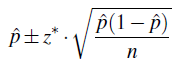
Now we’re done. The confidence interval for the population proportion p is:

\(\hat{p} \pm z^{*} \cdot \sqrt{\dfrac{\hat{p}(1-\hat{p})}{n}}\)

EXAMPLE:

The drug Viagra became available in the U.S. in May, 1998, in the wake of an advertising campaign that was unprecedented in scope and intensity. A Gallup poll found that by the end of the first week in May, 643 out of a random sample of 1,005 adults were aware that Viagra was an impotency medication (based on “Viagra A Popular Hit,” a Gallup poll analysis by Lydia Saad, May 1998).

Let’s estimate the proportion p of all adults in the U.S. who by the end of the first week of May 1998 were already aware of Viagra and its purpose by setting up a 95% confidence interval for p.

We first need to calculate the sample proportion p-hat. Out of 1,005 sampled adults, 643 knew what Viagra is used for, so p-hat = 643/1005 = 0.64

Therefore, a 95% confidence interval for p is

\begin{aligned}
\hat{p} \pm 1.96 \cdot \sqrt{\frac{\hat{p}(1-\hat{p})}{n}} &=0.64 \pm 1.96 \cdot \sqrt{\frac{0.64(1-0.64)}{1005}} \\
&=0.64 \pm 0.03 \\
&=(0.61,0.67)
\end{aligned}

We can be 95% confident that the proportion of all U.S. adults who were already familiar with Viagra by that time was between 0.61 and 0.67 (or 61% and 67%).

The fact that the margin of error equals 0.03 says we can be 95% confident that unknown population proportion p is within 0.03 (3%) of the observed sample proportion 0.64 (64%). In other words, we are 95% confident that 64% is “off” by no more than 3%.

Did I Get This?: Confidence Intervals – Proportions #1

Comment:

• We would like to share with you the methodology portion of the official poll release for the Viagra example. We hope you see that you now have the tools to understand how poll results are analyzed:

“The results are based on telephone interviews with a randomly selected national sample of 1,005 adults, 18 years and older, conducted May 8-10, 1998. For results based on samples of this size, one can say with 95 percent confidence that the error attributable to sampling and other random effects could be plus or minus 3 percentage points. In addition to sampling error, question wording and practical difficulties in conducting surveys can introduce error or bias into the findings of public opinion polls.”

The purpose of the next activity is to provide guided practice in calculating and interpreting the confidence interval for the population proportion p, and drawing conclusions from it.

Learn by Doing: Confidence Intervals – Proportions #1

Two important results that we discussed at length when we talked about the confidence interval for μ (mu) also apply here:

1. There is a trade-off between level of confidence and the width (or precision) of the confidence interval. The more precision you would like the confidence interval for p to have, the more you have to pay by having a lower level of confidence.

2. Since n appears in the denominator of the margin of error of the confidence interval for p, for a fixed level of confidence, the larger the sample, the narrower, or more precise it is. This brings us naturally to our next point.

Sample Size Calculations

Just as we did for means, when we have some level of flexibility in determining the sample size, we can set a desired margin of error for estimating the population proportion and find the sample size that will achieve that.

For example, a final poll on the day before an election would want the margin of error to be quite small (with a high level of confidence) in order to be able to predict the election results with the most precision. This is particularly relevant when it is a close race between the candidates. The polling company needs to figure out how many eligible voters it needs to include in their sample in order to achieve that.

Let’s see how we do that.

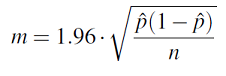
(Comment: For our discussion here we will focus on a 95% confidence level (z* = 1.96), since this is the most commonly used level of confidence.)

The confidence interval for p is

The margin of error, then, is

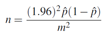
Now we isolate n (i.e., express it as a function of m).

There is a practical problem with this expression that we need to overcome.

Practically, you first determine the sample size, then you choose a random sample of that size, and then use the collected data to find p-hat.

So the fact that the expression above for determining the sample size depends on p-hat is problematic.

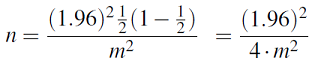
The way to overcome this problem is to take the conservative approach by setting p-hat = 1/2 = 0.5.

Why do we call this approach conservative?

It is conservative because the expression that appears in the numerator,

is maximized when p-hat = 1/2 = 0.5.

That way, the n we get will work in giving us the desired margin of error regardless of what the value of p-hat is. This is a “worst case scenario” approach. So when we do that we get:

In general, for any confidence level we have

• If we know a reasonable estimate of the proportion we can use:

\(n=\dfrac{\left(z^{*}\right)^{2} \hat{p}(1-\hat{p})}{m^{2}}\)

• If we choose the conservative estimate assuming we know nothing about the true proportion we use:

\(n=\dfrac{\left(z^{*}\right)^{2}}{4 \cdot m^{2}}\)

EXAMPLE:

It seems like media polls usually use a sample size of 1,000 to 1,200. This could be puzzling.

How could the results obtained from, say, 1,100 U.S. adults give us information about the entire population of U.S. adults? 1,100 is such a tiny fraction of the actual population. Here is the answer:

What sample size n is needed if a margin of error m = 0.03 is desired?

\(n=\dfrac{(1.96)^{2}}{4 \cdot(0.03)^{2}}=1067.1 \rightarrow 1068\)

(remember, always round up). In fact, 0.03 is a very commonly used margin of error, especially for media polls. For this reason, most media polls work with a sample of around 1,100 people.

Did I Get This?: Confidence Intervals – Proportions #2

When is it safe to use these methods?

As we mentioned before, one of the most important things to learn with any inference method is the conditions under which it is safe to use it.

As we did for the mean, the assumption we made in order to develop the methods in this unit was that the sampling distribution of the sample proportion, p-hat is roughly normal. Recall from the Probability unit that the conditions under which this happens are that

\(n p \geq 10 \text { and } n(1-p) \geq 10\)

Since p is unknown, we will replace it with its estimate, the sample proportion, and set

\(n \hat{p} \geq 10 \text { and } n(1-\hat{p}) \geq 10\)

to be the conditions under which it is safe to use the methods we developed in this section.

Here is one final practice for these confidence intervals!!

Did I Get This?: Confidence Intervals – Proportions #3

Let’s summarize

In general, a confidence interval for the unknown population proportion (p) is

\(\hat{p} \pm z^{*} \cdot \sqrt{\dfrac{\hat{p}(1-\hat{p})}{n}}\)

where z* is 1.645 for 90% confidence, 1.96 for 95% confidence, and 2.576 for 99% confidence.

To obtain a desired margin of error (m) in a confidence interval for an unknown population proportion, a conservative sample size is

\(n=\dfrac{\left(z^{*}\right)^{2}}{4 \cdot m^{2}}\)

If a reasonable estimate of the true proportion is known, the sample size can be calculated using

\(n = \dfrac{(1.96)^2 \hat{p} (1-\hat{p})}{m^2}\)

The methods developed in this unit are safe to use as long as

\(n \hat{p} \geq 10 \text{ and } n(1-\hat{p}) \geq 10\)

Wrap-Up (Estimation)

In this section on estimation, we have discussed the basic process for constructing confidence intervals from point estimates. In doing so we must calculate the margin of error using the standard error (or estimated standard error) and a z* or t* value.

As we wrap up this topic, we wanted to again discuss the interpretation of a confidence interval.

What do we mean by “confidence”?

Suppose we find a 95% confidence interval for an unknown parameter, what does the 95% mean exactly?

• If we repeat the process for all possible samples of this size for the population, 95% of the intervals we construct will contain the parameter

This is NOT the same as saying “the probability that μ (mu) is contained in (the interval constructed from my sample) is 95%.” Why?!

Answer

• Once we have a particular confidence interval, the true value is either in the interval constructed from our sample (probability = 1) or it is not (probability = 0). We simply do not know which it is. If we were to say “the probability that μ (mu) is contained in (the interval constructed from my sample) is 95%,” we know we would be incorrect since it is either 0 (No) or 1 (Yes) for any given sample. The probability comes from the “long run” view of the process.

• The probability we used to construct the confidence interval was based upon the fact that the sample statistic (x-bar, p-hat) will vary in a manner we understand (because we know the sampling distribution).

• The probability is associated with the randomness of our statistic so that for a particular interval we only speak of being “95% confident” which translates into an understanding about the process.

• In other words, in statistics, “95% confident” means our confidence in the process and implies that in the long run, we will be correct by using this process 95% of the time but that 5% of the time we will be incorrect. For one particular use of this process we cannot know if we are one of the 95% which are correct or one of the 5% which are incorrect. That is the statistical definition of confidence.

• We can say that in the long run, 95% of these intervals will contain the true parameter and 5% will not.

Correct Interpretations:

Example: Suppose a 95% confidence interval for the proportion of U.S. adults who are not active at all is (0.23, 0.27).

• Correct Interpretation #1: We are 95% confident that the true proportion of U.S. adults who are not active at all is between 23% and 27%

• Correct Interpretation #2: We are 95% confident that the true proportion of U.S. adults who are not active at all is covered by the interval (23%, 27%)

• A More Thorough Interpretation: Based upon our sample, the true proportion of U.S. adults who are not active at all is estimated to be 25%. With 95% confidence, this value could be as small as 23% to as large as 27%.

• A Common Interpretation in Journal Articles: Based upon our sample, the true proportion of U.S. adults who are not active at all is estimated to be 25% (95% CI 23%-27%).

Now let’s look at an INCORRECT interpretation which we have seen before

• INCORRECT Interpretation: There is a 95% chance that the true proportion of U.S. adults who are not active at all is between 23% and 27%. We know this is incorrect because at this point, the true proportion and the numbers in our interval are fixed. The probability is either 1 or 0 depending on whether the interval is one of the 95% that cover the true proportion, or one of the 5% that do not.

For confidence intervals regarding a population mean, we have an additional caution to discuss about interpretations.

Example: Suppose a 95% confidence interval for the average minutes per day of exercise for U.S. adults is (12, 18).

• Correct Interpretation: We are 95% confident that the true mean minutes per day of exercise for U.S. adults is between 12 and 18 minutes.

• INCORRECT Interpretation: We are 95% confident that an individual U.S. adult exercises between 12 and 18 minutes per day. We must remember that our intervals are about the parameter, in this case the population mean. They do not apply to an individual as we expect individuals to have much more variation.

• INCORRECT Interpretation: We are 95% confident that U.S. adults exercise between 12 and 18 minutes per day.This interpretation is implying this is true for all U.S. adults. This is an incorrect interpretation for the same reason as the previous incorrect interpretation!

As we continue to study inferential statistics, we will see that confidence intervals are used in many situations. The goal is always to provide confidence in our interval estimate of a quantity of interest. Population means and proportions are common parameters, however, any quantity that can be estimated from data has a population counterpart which we may wish to estimate.

(Optional) Outside Reading: Little Handbook – Confidence Intervals (and More) (4 Readings, ≈ 5500 words)