
Unit 3B: Sampling Distribution
- Page ID
- 31264
\( \newcommand{\vecs}[1]{\overset { \scriptstyle \rightharpoonup} {\mathbf{#1}} } \)
\( \newcommand{\vecd}[1]{\overset{-\!-\!\rightharpoonup}{\vphantom{a}\smash {#1}}} \)
\( \newcommand{\dsum}{\displaystyle\sum\limits} \)
\( \newcommand{\dint}{\displaystyle\int\limits} \)
\( \newcommand{\dlim}{\displaystyle\lim\limits} \)
\( \newcommand{\id}{\mathrm{id}}\) \( \newcommand{\Span}{\mathrm{span}}\)
( \newcommand{\kernel}{\mathrm{null}\,}\) \( \newcommand{\range}{\mathrm{range}\,}\)
\( \newcommand{\RealPart}{\mathrm{Re}}\) \( \newcommand{\ImaginaryPart}{\mathrm{Im}}\)
\( \newcommand{\Argument}{\mathrm{Arg}}\) \( \newcommand{\norm}[1]{\| #1 \|}\)
\( \newcommand{\inner}[2]{\langle #1, #2 \rangle}\)
\( \newcommand{\Span}{\mathrm{span}}\)
\( \newcommand{\id}{\mathrm{id}}\)
\( \newcommand{\Span}{\mathrm{span}}\)
\( \newcommand{\kernel}{\mathrm{null}\,}\)
\( \newcommand{\range}{\mathrm{range}\,}\)
\( \newcommand{\RealPart}{\mathrm{Re}}\)
\( \newcommand{\ImaginaryPart}{\mathrm{Im}}\)
\( \newcommand{\Argument}{\mathrm{Arg}}\)
\( \newcommand{\norm}[1]{\| #1 \|}\)
\( \newcommand{\inner}[2]{\langle #1, #2 \rangle}\)
\( \newcommand{\Span}{\mathrm{span}}\) \( \newcommand{\AA}{\unicode[.8,0]{x212B}}\)
\( \newcommand{\vectorA}[1]{\vec{#1}} % arrow\)
\( \newcommand{\vectorAt}[1]{\vec{\text{#1}}} % arrow\)
\( \newcommand{\vectorB}[1]{\overset { \scriptstyle \rightharpoonup} {\mathbf{#1}} } \)
\( \newcommand{\vectorC}[1]{\textbf{#1}} \)
\( \newcommand{\vectorD}[1]{\overrightarrow{#1}} \)
\( \newcommand{\vectorDt}[1]{\overrightarrow{\text{#1}}} \)
\( \newcommand{\vectE}[1]{\overset{-\!-\!\rightharpoonup}{\vphantom{a}\smash{\mathbf {#1}}}} \)
\( \newcommand{\vecs}[1]{\overset { \scriptstyle \rightharpoonup} {\mathbf{#1}} } \)
\(\newcommand{\longvect}{\overrightarrow}\)
\( \newcommand{\vecd}[1]{\overset{-\!-\!\rightharpoonup}{\vphantom{a}\smash {#1}}} \)
\(\newcommand{\avec}{\mathbf a}\) \(\newcommand{\bvec}{\mathbf b}\) \(\newcommand{\cvec}{\mathbf c}\) \(\newcommand{\dvec}{\mathbf d}\) \(\newcommand{\dtil}{\widetilde{\mathbf d}}\) \(\newcommand{\evec}{\mathbf e}\) \(\newcommand{\fvec}{\mathbf f}\) \(\newcommand{\nvec}{\mathbf n}\) \(\newcommand{\pvec}{\mathbf p}\) \(\newcommand{\qvec}{\mathbf q}\) \(\newcommand{\svec}{\mathbf s}\) \(\newcommand{\tvec}{\mathbf t}\) \(\newcommand{\uvec}{\mathbf u}\) \(\newcommand{\vvec}{\mathbf v}\) \(\newcommand{\wvec}{\mathbf w}\) \(\newcommand{\xvec}{\mathbf x}\) \(\newcommand{\yvec}{\mathbf y}\) \(\newcommand{\zvec}{\mathbf z}\) \(\newcommand{\rvec}{\mathbf r}\) \(\newcommand{\mvec}{\mathbf m}\) \(\newcommand{\zerovec}{\mathbf 0}\) \(\newcommand{\onevec}{\mathbf 1}\) \(\newcommand{\real}{\mathbb R}\) \(\newcommand{\twovec}[2]{\left[\begin{array}{r}#1 \\ #2 \end{array}\right]}\) \(\newcommand{\ctwovec}[2]{\left[\begin{array}{c}#1 \\ #2 \end{array}\right]}\) \(\newcommand{\threevec}[3]{\left[\begin{array}{r}#1 \\ #2 \\ #3 \end{array}\right]}\) \(\newcommand{\cthreevec}[3]{\left[\begin{array}{c}#1 \\ #2 \\ #3 \end{array}\right]}\) \(\newcommand{\fourvec}[4]{\left[\begin{array}{r}#1 \\ #2 \\ #3 \\ #4 \end{array}\right]}\) \(\newcommand{\cfourvec}[4]{\left[\begin{array}{c}#1 \\ #2 \\ #3 \\ #4 \end{array}\right]}\) \(\newcommand{\fivevec}[5]{\left[\begin{array}{r}#1 \\ #2 \\ #3 \\ #4 \\ #5 \\ \end{array}\right]}\) \(\newcommand{\cfivevec}[5]{\left[\begin{array}{c}#1 \\ #2 \\ #3 \\ #4 \\ #5 \\ \end{array}\right]}\) \(\newcommand{\mattwo}[4]{\left[\begin{array}{rr}#1 \amp #2 \\ #3 \amp #4 \\ \end{array}\right]}\) \(\newcommand{\laspan}[1]{\text{Span}\{#1\}}\) \(\newcommand{\bcal}{\cal B}\) \(\newcommand{\ccal}{\cal C}\) \(\newcommand{\scal}{\cal S}\) \(\newcommand{\wcal}{\cal W}\) \(\newcommand{\ecal}{\cal E}\) \(\newcommand{\coords}[2]{\left\{#1\right\}_{#2}}\) \(\newcommand{\gray}[1]{\color{gray}{#1}}\) \(\newcommand{\lgray}[1]{\color{lightgray}{#1}}\) \(\newcommand{\rank}{\operatorname{rank}}\) \(\newcommand{\row}{\text{Row}}\) \(\newcommand{\col}{\text{Col}}\) \(\renewcommand{\row}{\text{Row}}\) \(\newcommand{\nul}{\text{Nul}}\) \(\newcommand{\var}{\text{Var}}\) \(\newcommand{\corr}{\text{corr}}\) \(\newcommand{\len}[1]{\left|#1\right|}\) \(\newcommand{\bbar}{\overline{\bvec}}\) \(\newcommand{\bhat}{\widehat{\bvec}}\) \(\newcommand{\bperp}{\bvec^\perp}\) \(\newcommand{\xhat}{\widehat{\xvec}}\) \(\newcommand{\vhat}{\widehat{\vvec}}\) \(\newcommand{\uhat}{\widehat{\uvec}}\) \(\newcommand{\what}{\widehat{\wvec}}\) \(\newcommand{\Sighat}{\widehat{\Sigma}}\) \(\newcommand{\lt}{<}\) \(\newcommand{\gt}{>}\) \(\newcommand{\amp}{&}\) \(\definecolor{fillinmathshade}{gray}{0.9}\)CO-6: Apply basic concepts of probability, random variation, and commonly used statistical probability distributions.
NOTE: The following videos discuss all three pages related to sampling distributions.
Review: We will apply the concepts of normal random variables to two random variables which are summary statistics from a sample – these are the sample mean (x-bar) and the sample proportion (p-hat).
Video: Sampling Distributions (34:00 total time)
Introduction
Already on several occasions we have pointed out the important distinction between a population and a sample. In Exploratory Data Analysis, we learned to summarize and display values of a variable for a sample, such as displaying the blood types of 100 randomly chosen U.S. adults using a pie chart, or displaying the heights of 150 males using a histogram and supplementing it with appropriate numerical measures such as the sample mean (x-bar) and sample standard deviation (s).
In our study of Probability and Random Variables, we discussed the long-run behavior of a variable, considering the population of all possible values taken by that variable. For example, we talked about the distribution of blood types among all U.S. adults and the distribution of the random variable X, representing a male’s height.
Now we focus directly on the relationship between the values of a variable for a sample and its values for the entire population from which the sample was taken. This material is the bridge between probability and our ultimate goal of the course, statistical inference. In inference, we look at a sample and ask what we can say about the population from which it was drawn.
Now, we’ll pose the reverse question: If I know what the population looks like, what can I expect the sample to look like? Clearly, inference poses the more practical question, since in practice we can look at a sample, but rarely do we know what the whole population looks like. This material will be more theoretical in nature, since it poses a problem which is not really practical, but will present important ideas which are the foundation for statistical inference.
Parameters vs. Statistics
LO 6.19: Identify and distinguish between a parameter and a statistic.
LO 6.20: Explain the concepts of sampling variability and sampling distribution.
To better understand the relationship between sample and population, let’s consider the two examples that were mentioned in the introduction.
In the probability section, we presented the distribution of blood types in the entire U.S. population:
Assume now that we take a sample of 500 people in the United States, record their blood type, and display the sample results:
Note that the percentages (or proportions) that we found in our sample are slightly different than the population percentages. This is really not surprising. Since we took a sample of just 500, we cannot expect that our sample will behave exactly like the population, but if the sample is random (as it was), we expect to get results which are not that far from the population (as we did). If we took yet another sample of size 500:
we again get sample results that are slightly different from the population figures, and also different from what we found in the first sample. This very intuitive idea, that sample results change from sample to sample, is called sampling variability.
Let’s look at another example:
Heights among the population of all adult males follow a normal distribution with a mean μ = mu =69 inches and a standard deviation σ = sigma =2.8 inches. Here is a probability display of this population distribution:
A sample of 200 males was chosen, and their heights were recorded. Here are the sample results:
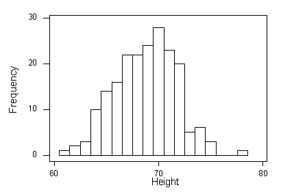
The sample mean (x-bar) is 68.7 inches and the sample standard deviation (s) is 2.95 inches.
Again, note that the sample results are slightly different from the population. The histogram for this sample resembles the normal distribution, but is not as fine, and also the sample mean and standard deviation are slightly different from the population mean and standard deviation. Let’s take another sample of 200 males:
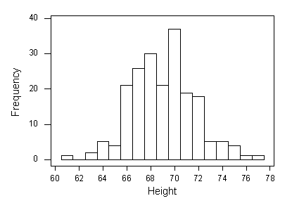
The sample mean (x-bar) is 69.1 inches and the sample standard deviation (s) is 2.66 inches.
Again, as in Example 1 we see the idea of sampling variability. In this second sample, the results are pretty close to the population, but different from the results we found in the first sample.
In both the examples, we have numbers that describe the population, and numbers that describe the sample. In Example 1, the number 42% is the population proportion of blood type A, and 39.6% is the sample proportion (in sample 1) of blood type A. In Example 2, 69 and 2.8 are the population mean and standard deviation, and (in sample 1) 68.7 and 2.95 are the sample mean and standard deviation.
A parameter is a number that describes the population.
A statistic is a number that is computed from the sample.
In Example 1: 42% (0.42) is the parameter and 39.6% (0.396) is a statistic (and 43.2% is another statistic).
In Example 2: 69 and 2.8 are the parameters and 68.7 and 2.95 are statistics (69.1 and 2.66 are also statistics).
In this course, as in the examples above, we focus on the following parameters and statistics:
- population proportion and sample proportion
- population mean and sample mean
- population standard deviation and sample standard deviation
The following table summarizes the three pairs, and gives the notation
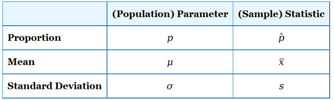
The only new notation here is p for population proportion (p = 0.42 for type A in Example 1), and p-hat (using the “hat” symbol ∧ over the p) for the sample proportion which is 0.396 in Example 1, sample 1).
Comments:
- Parameters are usually unknown, because it is impractical or impossible to know exactly what values a variable takes for every member of the population.
- Statistics are computed from the sample, and vary from sample to sample due to sampling variability.
In the last part of the course, statistical inference, we will learn how to use a statistic to draw conclusions about an unknown parameter, either by estimating it or by deciding whether it is reasonable to conclude that the parameter equals a proposed value.
Now we’ll learn about the behavior of the statistics assuming that we know the parameters. So, for example, if we know that the population proportion of blood type A in the population is 0.42, and we take a random sample of size 500, what do we expect the sample proportion p-hat to be? Specifically we ask:
- What is the distribution of all possible sample proportions from samples of size 500?
- Where is it centered?
- How much variation exists among different sample proportions from samples of size 500?
- How far off the true value of 0.42 might we expect to be?
Here are some more examples:
If students picked numbers completely at random from the numbers 1 to 20, the proportion of times that the number 7 would be picked is 0.05. When 15 students picked a number “at random” from 1 to 20, 3 of them picked the number 7. Identify the parameter and accompanying statistic in this situation.
The parameter is the population proportion of random selections resulting in the number 7, which is p = 0.05. The accompanying statistic is the sample proportion (p-hat) of selections resulting in the number 7, which is 3/15=0.20.
Note: Unrelated to our current discussion, this is an interesting illustration of how we (humans) are not very good at doing things randomly. I used to ask a similar question in introductory statistics courses where I asked students to RANDOMLY pick a number between 1 and 10. The number of students choosing 7 is almost always MUCH larger than would be predicted if the results were truly random.
Try it with some of your friends and family and see if you get similar results. We really like the number 7! Interestingly, if students were aware of this phenomenon, then they tended to pick 3 most often. This is interesting since if choices were truly random, we should see a relatively equal proportion for each number :-)
The length of human pregnancies has a mean of 266 days and a standard deviation of 16 days. A random sample of 9 pregnant women was observed to have a mean pregnancy length of 270 days, with a standard deviation of 14 days. Identify the parameters and accompanying statistics in this situation.
The parameters are population mean μ = mu =266 and population standard deviation σ = sigma = 16. The accompanying statistics are sample mean (x-bar) = 270 and sample standard deviation (s) = 14.
The first step to drawing conclusions about parameters based on the accompanying statistics is to understand how sample statistics behave relative to the parameter(s) that summarizes the entire population. We begin with the behavior of sample proportion relative to population proportion (when the variable of interest is categorical). After that, we will explore the behavior of sample mean relative to population mean (when the variable of interest is quantitative).
Did I Get This?: Parameters vs. Statistics