13.2: Prediction

The goal of regression is the same as the goal of ANOVA: to take what we know about one variable (\(X\)) and use it to explain our observed differences in another variable (\(Y\)). In ANOVA, we talked about – and tested for – group mean differences, but in regression we do not have groups for our explanatory variable; we have a continuous variable, like in correlation. Because of this, our vocabulary will be a little bit different, but the process, logic, and end result are all the same.

In regression, we most frequently talk about prediction, specifically predicting our outcome variable \(Y\) from our explanatory variable \(X\), and we use the line of best fit to make our predictions. Let’s take a look at the equation for the line, which is quite simple:

\[\widehat{\mathrm{Y}}=\mathrm{a}+\mathrm{bX} \]

The terms in the equation are defined as:

• \(\widehat{\mathrm{Y}}\): the predicted value of \(Y\) for an individual person
• \(a\): the intercept of the line
• \(b\): the slope of the line
• \(X\): the observed value of \(X\) for an individual person

What this shows us is that we will use our known value of \(X\) for each person to predict the value of \(Y\) for that person. The predicted value, \(\widehat{\mathrm{Y}}\), is called “\(y\)-hat” and is our best guess for what a person’s score on the outcome is. Notice also that the form of the equation is very similar to very simple linear equations that you have likely encountered before and has only two parameter estimates: an intercept (where the line crosses the Y-axis) and a slope (how steep – and the direction, positive or negative – the line is). These are parameter estimates because, like everything else in statistics, we are interested in approximating the true value of the relation in the population but can only ever estimate it using sample data. We will soon see that one of these parameters, the slope, is the focus of our hypothesis tests (the intercept is only there to make the math work out properly and is rarely interpretable). The formulae for these parameter estimates use very familiar values:

\[\mathrm{a}=\overline{\mathrm{Y}}-\mathrm{b} \overline{\mathrm{X}} \]

\[\mathrm{b}=\dfrac{\operatorname{cov}_{X Y}}{s_{X}^{2}}=\dfrac{S P}{S S X}=r\left(\dfrac{S_{y}}{s_{x}}\right) \]

We have seen each of these before. \(\overline{Y}\) and \(\overline{X}\) are the means of \(Y\) and \(X\), respectively; \(\operatorname{cov}_{X Y}\) is the covariance of \(X\) and \(Y\) we learned about with correlations; and \(s_{X}^{2}\) is the variance of \(X\). The formula for the slope is very similar to the formula for a Pearson correlation coefficient; the only difference is that we are dividing by the variance of \(X\) instead of the product of the standard deviations of \(X\) and \(Y\). Because of this, our slope is scaled to the same scale as our \(X\) variable and is no longer constrained to be between 0 and 1 in absolute value. This formula provides a clear definition of the slope of the line of best fit, and just like with correlation, this definitional formula can be simplified into a short computational formula for easier calculations. In this case, we are simply taking the sum of products and dividing by the sum of squares for \(X\).

Notice that there is a third formula for the slope of the line that involves the correlation between \(X\) and \(Y\). This is because regression and correlation look for the same thing: a straight line through the middle of the data. The only difference between a regression coefficient in simple linear regression and a Pearson correlation coefficient is the scale. So, if you lack raw data but have summary information on the correlation and standard deviations for variables, you can still compute a slope, and therefore intercept, for a line of best fit.

It is very important to point out that the \(Y\) values in the equations for \(a\) and \(b\) are our observed \(Y\) values in the dataset, NOT the predicted \(Y\) values (\(\widehat{\mathrm{Y}}\)) from our equation for the line of best fit. Thus, we will have 3 values for each person: the observed value of \(X (X)\), the observed value of \(Y (Y)\), and the predicted value of \(Y (\widehat{\mathrm{Y}}\)). You may be asking why we would try to predict \(Y\) if we have an observed value of \(Y\), and that is a very reasonable question. The answer has two explanations: first, we need to use known values of \(Y\) to calculate the parameter estimates in our equation, and we use the difference between our observed values and predicted values (\(Y – \widehat{\mathrm{Y}}\)) to see how accurate our equation is; second, we often use regression to create a predictive model that we can then use to predict values of \(Y\) for other people for whom we only have information on \(X\).

Let’s look at this from an applied example. Businesses often have more applicants for a job than they have openings available, so they want to know who among the applicants is most likely to be the best employee. There are many criteria that can be used, but one is a personality test for conscientiousness, with the belief being that more conscientious (more responsible) employees are better than less conscientious employees. A business might give their employees a personality inventory to assess conscientiousness and existing performance data to look for a relation. In this example, we have known values of the predictor (\(X\), conscientiousness) and outcome (\(Y\), job performance), so we can estimate an equation for a line of best fit and see how accurately conscientious predicts job performance, then use this equation to predict future job performance of applicants based only on their known values of conscientiousness from personality inventories given during the application process.

The key assessing whether a linear regression works well is the difference between our observed and known \(Y\) values and our predicted \(\widehat{\mathrm{Y}}\) values. As mentioned in passing above, we use subtraction to find the difference between them (\(Y – \widehat{\mathrm{Y}}\)) in the same way we use subtraction for deviation scores and sums of squares. The value (\(Y – \widehat{\mathrm{Y}}\)) is our residual, which, as defined above, is how close our line of best fit is to our actual values. We can visualize residuals to get a better sense of what they are by creating a scatterplot and overlaying a line of best fit on it, as shown in Figure \(\PageIndex{1}\).

Figure \(\PageIndex{1}\): Scatterplot with residuals.

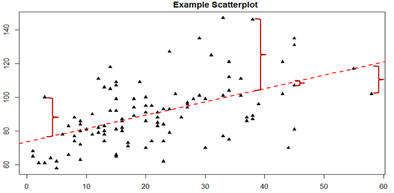
In Figure \(\PageIndex{1}\), the triangular dots represent observations from each person on both \(X\) and \(Y\) and the dashed bright red line is the line of best fit estimated by the equation \(\widehat{\mathrm{Y}}= a + bX\). For every person in the dataset, the line represents their predicted score. The dark red bracket between the triangular dots and the predicted scores on the line of best fit are our residuals (they are only drawn for four observations for ease of viewing, but in reality there is one for every observation); you can see that some residuals are positive and some are negative, and that some are very large and some are very small. This means that some predictions are very accurate and some are very inaccurate, and the some predictions overestimated values and some underestimated values. Across the entire dataset, the line of best fit is the one that minimizes the total (sum) value of all residuals. That is, although predictions at an individual level might be somewhat inaccurate, across our full sample and (theoretically) in future samples our total amount of error is as small as possible. We call this property of the line of best fit the Least Squares Error Solution. This term means that the solution – or equation – of the line is the one that provides the smallest possible value of the squared errors (squared so that they can be summed, just like in standard deviation) relative to any other straight line we could draw through the data.

Predicting Scores and Explaining Variance

We have now seen that the purpose of regression is twofold: we want to predict scores based on our line and, as stated earlier, explain variance in our observed \(Y\) variable just like in ANOVA. These two purposes go hand in hand, and our ability to predict scores is literally our ability to explain variance. That is, if we cannot account for the variance in \(Y\) based on \(X\), then we have no reason to use \(X\) to predict future values of \(Y\).

We know that the overall variance in \(Y\) is a function of each score deviating from the mean of \(Y\) (as in our calculation of variance and standard deviation). So, just like the red brackets in figure 1 representing residuals, given as (\(Y – \widehat{\mathrm{Y}}\)), we can visualize the overall variance as each score’s distance from the overall mean of \(Y\), given as (\(Y – \overline{Y}\)), our normal deviation score. This is shown in Figure \(\PageIndex{2}\).

Figure \(\PageIndex{2}\): Scatterplot with residuals and deviation scores.

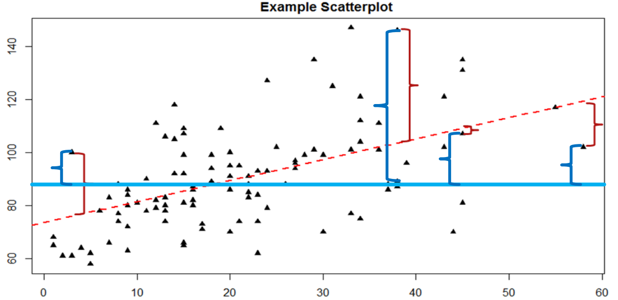
In Figure \(\PageIndex{2}\), the solid blue line is the mean of \(Y\), and the blue brackets are the deviation scores between our observed values of \(Y\) and the mean of \(Y\). This represents the overall variance that we are trying to explain. Thus, the residuals and the deviation scores are the same type of idea: the distance between an observed score and a given line, either the line of best fit that gives predictions or the line representing the mean that serves as a baseline. The difference between these two values, which is the distance between the lines themselves, is our model’s ability to predict scores above and beyond the baseline mean; that is, it is our models ability to explain the variance we observe in \(Y\) based on values of \(X\). If we have no ability to explain variance, then our line will be flat (the slope will be 0.00) and will be the same as the line representing the mean, and the distance between the lines will be 0.00 as well.

We now have three pieces of information: the distance from the observed score to the mean, the distance from the observed score to the prediction line, and the distance from the prediction line to the mean. These are our three pieces of information needed to test our hypotheses about regression and to calculate effect sizes. They are our three Sums of Squares, just like in ANOVA. Our distance from the observed score to the mean is the Sum of Squares Total, which we are trying to explain. Our distance from the observed score to the prediction line is our Sum of Squares Error, or residual, which we are trying to minimize. Our distance from the prediction line to the mean is our Sum of Squares Model, which is our observed effect and our ability to explain variance. Each of these will go into the ANOVA table to calculate our test statistic.