
8.2: Hypothesis Testing with t
- Page ID
- 7127

\( \newcommand{\vecs}[1]{\overset { \scriptstyle \rightharpoonup} {\mathbf{#1}} } \)
\( \newcommand{\vecd}[1]{\overset{-\!-\!\rightharpoonup}{\vphantom{a}\smash {#1}}} \)
\( \newcommand{\id}{\mathrm{id}}\) \( \newcommand{\Span}{\mathrm{span}}\)
( \newcommand{\kernel}{\mathrm{null}\,}\) \( \newcommand{\range}{\mathrm{range}\,}\)
\( \newcommand{\RealPart}{\mathrm{Re}}\) \( \newcommand{\ImaginaryPart}{\mathrm{Im}}\)
\( \newcommand{\Argument}{\mathrm{Arg}}\) \( \newcommand{\norm}[1]{\| #1 \|}\)
\( \newcommand{\inner}[2]{\langle #1, #2 \rangle}\)
\( \newcommand{\Span}{\mathrm{span}}\)
\( \newcommand{\id}{\mathrm{id}}\)
\( \newcommand{\Span}{\mathrm{span}}\)
\( \newcommand{\kernel}{\mathrm{null}\,}\)
\( \newcommand{\range}{\mathrm{range}\,}\)
\( \newcommand{\RealPart}{\mathrm{Re}}\)
\( \newcommand{\ImaginaryPart}{\mathrm{Im}}\)
\( \newcommand{\Argument}{\mathrm{Arg}}\)
\( \newcommand{\norm}[1]{\| #1 \|}\)
\( \newcommand{\inner}[2]{\langle #1, #2 \rangle}\)
\( \newcommand{\Span}{\mathrm{span}}\) \( \newcommand{\AA}{\unicode[.8,0]{x212B}}\)
\( \newcommand{\vectorA}[1]{\vec{#1}} % arrow\)
\( \newcommand{\vectorAt}[1]{\vec{\text{#1}}} % arrow\)
\( \newcommand{\vectorB}[1]{\overset { \scriptstyle \rightharpoonup} {\mathbf{#1}} } \)
\( \newcommand{\vectorC}[1]{\textbf{#1}} \)
\( \newcommand{\vectorD}[1]{\overrightarrow{#1}} \)
\( \newcommand{\vectorDt}[1]{\overrightarrow{\text{#1}}} \)
\( \newcommand{\vectE}[1]{\overset{-\!-\!\rightharpoonup}{\vphantom{a}\smash{\mathbf {#1}}}} \)
\( \newcommand{\vecs}[1]{\overset { \scriptstyle \rightharpoonup} {\mathbf{#1}} } \)
\( \newcommand{\vecd}[1]{\overset{-\!-\!\rightharpoonup}{\vphantom{a}\smash {#1}}} \)
\(\newcommand{\avec}{\mathbf a}\) \(\newcommand{\bvec}{\mathbf b}\) \(\newcommand{\cvec}{\mathbf c}\) \(\newcommand{\dvec}{\mathbf d}\) \(\newcommand{\dtil}{\widetilde{\mathbf d}}\) \(\newcommand{\evec}{\mathbf e}\) \(\newcommand{\fvec}{\mathbf f}\) \(\newcommand{\nvec}{\mathbf n}\) \(\newcommand{\pvec}{\mathbf p}\) \(\newcommand{\qvec}{\mathbf q}\) \(\newcommand{\svec}{\mathbf s}\) \(\newcommand{\tvec}{\mathbf t}\) \(\newcommand{\uvec}{\mathbf u}\) \(\newcommand{\vvec}{\mathbf v}\) \(\newcommand{\wvec}{\mathbf w}\) \(\newcommand{\xvec}{\mathbf x}\) \(\newcommand{\yvec}{\mathbf y}\) \(\newcommand{\zvec}{\mathbf z}\) \(\newcommand{\rvec}{\mathbf r}\) \(\newcommand{\mvec}{\mathbf m}\) \(\newcommand{\zerovec}{\mathbf 0}\) \(\newcommand{\onevec}{\mathbf 1}\) \(\newcommand{\real}{\mathbb R}\) \(\newcommand{\twovec}[2]{\left[\begin{array}{r}#1 \\ #2 \end{array}\right]}\) \(\newcommand{\ctwovec}[2]{\left[\begin{array}{c}#1 \\ #2 \end{array}\right]}\) \(\newcommand{\threevec}[3]{\left[\begin{array}{r}#1 \\ #2 \\ #3 \end{array}\right]}\) \(\newcommand{\cthreevec}[3]{\left[\begin{array}{c}#1 \\ #2 \\ #3 \end{array}\right]}\) \(\newcommand{\fourvec}[4]{\left[\begin{array}{r}#1 \\ #2 \\ #3 \\ #4 \end{array}\right]}\) \(\newcommand{\cfourvec}[4]{\left[\begin{array}{c}#1 \\ #2 \\ #3 \\ #4 \end{array}\right]}\) \(\newcommand{\fivevec}[5]{\left[\begin{array}{r}#1 \\ #2 \\ #3 \\ #4 \\ #5 \\ \end{array}\right]}\) \(\newcommand{\cfivevec}[5]{\left[\begin{array}{c}#1 \\ #2 \\ #3 \\ #4 \\ #5 \\ \end{array}\right]}\) \(\newcommand{\mattwo}[4]{\left[\begin{array}{rr}#1 \amp #2 \\ #3 \amp #4 \\ \end{array}\right]}\) \(\newcommand{\laspan}[1]{\text{Span}\{#1\}}\) \(\newcommand{\bcal}{\cal B}\) \(\newcommand{\ccal}{\cal C}\) \(\newcommand{\scal}{\cal S}\) \(\newcommand{\wcal}{\cal W}\) \(\newcommand{\ecal}{\cal E}\) \(\newcommand{\coords}[2]{\left\{#1\right\}_{#2}}\) \(\newcommand{\gray}[1]{\color{gray}{#1}}\) \(\newcommand{\lgray}[1]{\color{lightgray}{#1}}\) \(\newcommand{\rank}{\operatorname{rank}}\) \(\newcommand{\row}{\text{Row}}\) \(\newcommand{\col}{\text{Col}}\) \(\renewcommand{\row}{\text{Row}}\) \(\newcommand{\nul}{\text{Nul}}\) \(\newcommand{\var}{\text{Var}}\) \(\newcommand{\corr}{\text{corr}}\) \(\newcommand{\len}[1]{\left|#1\right|}\) \(\newcommand{\bbar}{\overline{\bvec}}\) \(\newcommand{\bhat}{\widehat{\bvec}}\) \(\newcommand{\bperp}{\bvec^\perp}\) \(\newcommand{\xhat}{\widehat{\xvec}}\) \(\newcommand{\vhat}{\widehat{\vvec}}\) \(\newcommand{\uhat}{\widehat{\uvec}}\) \(\newcommand{\what}{\widehat{\wvec}}\) \(\newcommand{\Sighat}{\widehat{\Sigma}}\) \(\newcommand{\lt}{<}\) \(\newcommand{\gt}{>}\) \(\newcommand{\amp}{&}\) \(\definecolor{fillinmathshade}{gray}{0.9}\)Hypothesis testing with the \(t\)-statistic works exactly the same way as \(z\)-tests did, following the four-step process of
- Stating the Hypothesis
- Finding the Critical Values
- Computing the Test Statistic
- Making the Decision.
We will work though an example: let’s say that you move to a new city and find a an auto shop to change your oil. Your old mechanic did the job in about 30 minutes (though you never paid close enough attention to know how much that varied), and you suspect that your new shop takes much longer. After 4 oil changes, you think you have enough evidence to demonstrate this.
Step 1: State the Hypotheses Our hypotheses for 1-sample t-tests are identical to those we used for \(z\)-tests. We still state the null and alternative hypotheses mathematically in terms of the population parameter and written out in readable English. For our example:
\(H_0\): There is no difference in the average time to change a car’s oil
\(H_0: μ = 30\)
\(H_A\): This shop takes longer to change oil than your old mechanic
\(H_A: μ > 30\)
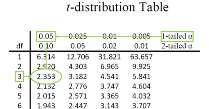
Step 2: Find the Critical Values As noted above, our critical values still delineate the area in the tails under the curve corresponding to our chosen level of significance. Because we have no reason to change significance levels, we will use \(α\) = 0.05, and because we suspect a direction of effect, we have a one-tailed test. To find our critical values for \(t\), we need to add one more piece of information: the degrees of freedom. For this example:
\[df = N – 1 = 4 – 1 = 3 \nonumber \]
Going to our \(t\)-table, we find the column corresponding to our one-tailed significance level and find where it intersects with the row for 3 degrees of freedom. As shown in Figure \(\PageIndex{1}\): our critical value is \(t*\) = 2.353
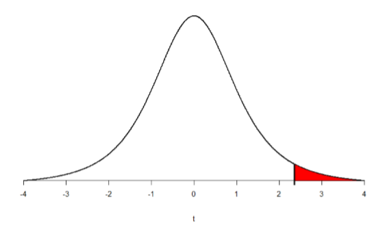
We can then shade this region on our \(t\)-distribution to visualize our rejection region
Step 3: Compute the Test Statistic The four wait times you experienced for your oil changes are the new shop were 46 minutes, 58 minutes, 40 minutes, and 71 minutes. We will use these to calculate \(\overline{\mathrm{X}}\) and s by first filling in the sum of squares table in Table \(\PageIndex{1}\):
| \(\overline{\mathrm{X}}\) | \(\mathrm{X}-\overline{\mathrm{X}}\) | \((\mathrm{X}-\overline{\mathrm{X}})^{2}\) |
|---|---|---|
| 46 | -7.75 | 60.06 |
| 58 | 4.25 | 18.06 |
| 40 | -13.75 | 189.06 |
| 71 | 17.25 | 297.56 |
| \(\Sigma\)=215 | \(\Sigma\)=0 | \(\Sigma\)=564.74 |
After filling in the first row to get \(\Sigma\)=215, we find that the mean is \(\overline{\mathrm{X}}\) = 53.75 (215 divided by sample size 4), which allows us to fill in the rest of the table to get our sum of squares \(SS\) = 564.74, which we then plug in to the formula for standard deviation from chapter 3:
\[s=\sqrt{\dfrac{\sum(X-\overline{X})^{2}}{N-1}}=\sqrt{\dfrac{S S}{d f}}=\sqrt{\dfrac{564.74}{3}}=13.72 \nonumber \]
Next, we take this value and plug it in to the formula for standard error:
\[s_{\overline{X}}=\dfrac{s}{\sqrt{n}}=\dfrac{13.72}{2}=6.86 \nonumber \]
And, finally, we put the standard error, sample mean, and null hypothesis value into the formula for our test statistic \(t\):
\[t=\dfrac{\overline{\mathrm{X}}-\mu}{s_{\overline{\mathrm{X}}}}=\dfrac{53.75-30}{6.86}=\dfrac{23.75}{6.68}=3.46 \nonumber \]
This may seem like a lot of steps, but it is really just taking our raw data to calculate one value at a time and carrying that value forward into the next equation: data sample size/degrees of freedom mean sum of squares standard deviation standard error test statistic. At each step, we simply match the symbols of what we just calculated to where they appear in the next formula to make sure we are plugging everything in correctly.
Step 4: Make the Decision Now that we have our critical value and test statistic, we can make our decision using the same criteria we used for a \(z\)-test. Our obtained \(t\)-statistic was \(t\) = 3.46 and our critical value was \(t* = 2.353: t > t*\), so we reject the null hypothesis and conclude:
Based on our four oil changes, the new mechanic takes longer on average (\(\overline{\mathrm{X}}\) = 53.75) to change oil than our old mechanic, \(t(3)\) = 3.46, \(p\) < .05.
Notice that we also include the degrees of freedom in parentheses next to \(t\). And because we found a significant result, we need to calculate an effect size, which is still Cohen’s \(d\), but now we use \(s\) in place of \(σ\):
\[d=\dfrac{\overline{X}-\mu}{s}=\dfrac{53.75-30.00}{13.72}=1.73 \nonumber \]
This is a large effect. It should also be noted that for some things, like the minutes in our current example, we can also interpret the magnitude of the difference we observed (23 minutes and 45 seconds) as an indicator of importance since time is a familiar metric.