1.1: Introduction and Examples
- Page ID
- 832
\( \newcommand{\vecs}[1]{\overset { \scriptstyle \rightharpoonup} {\mathbf{#1}} } \)
\( \newcommand{\vecd}[1]{\overset{-\!-\!\rightharpoonup}{\vphantom{a}\smash {#1}}} \)
\( \newcommand{\dsum}{\displaystyle\sum\limits} \)
\( \newcommand{\dint}{\displaystyle\int\limits} \)
\( \newcommand{\dlim}{\displaystyle\lim\limits} \)
\( \newcommand{\id}{\mathrm{id}}\) \( \newcommand{\Span}{\mathrm{span}}\)
( \newcommand{\kernel}{\mathrm{null}\,}\) \( \newcommand{\range}{\mathrm{range}\,}\)
\( \newcommand{\RealPart}{\mathrm{Re}}\) \( \newcommand{\ImaginaryPart}{\mathrm{Im}}\)
\( \newcommand{\Argument}{\mathrm{Arg}}\) \( \newcommand{\norm}[1]{\| #1 \|}\)
\( \newcommand{\inner}[2]{\langle #1, #2 \rangle}\)
\( \newcommand{\Span}{\mathrm{span}}\)
\( \newcommand{\id}{\mathrm{id}}\)
\( \newcommand{\Span}{\mathrm{span}}\)
\( \newcommand{\kernel}{\mathrm{null}\,}\)
\( \newcommand{\range}{\mathrm{range}\,}\)
\( \newcommand{\RealPart}{\mathrm{Re}}\)
\( \newcommand{\ImaginaryPart}{\mathrm{Im}}\)
\( \newcommand{\Argument}{\mathrm{Arg}}\)
\( \newcommand{\norm}[1]{\| #1 \|}\)
\( \newcommand{\inner}[2]{\langle #1, #2 \rangle}\)
\( \newcommand{\Span}{\mathrm{span}}\) \( \newcommand{\AA}{\unicode[.8,0]{x212B}}\)
\( \newcommand{\vectorA}[1]{\vec{#1}} % arrow\)
\( \newcommand{\vectorAt}[1]{\vec{\text{#1}}} % arrow\)
\( \newcommand{\vectorB}[1]{\overset { \scriptstyle \rightharpoonup} {\mathbf{#1}} } \)
\( \newcommand{\vectorC}[1]{\textbf{#1}} \)
\( \newcommand{\vectorD}[1]{\overrightarrow{#1}} \)
\( \newcommand{\vectorDt}[1]{\overrightarrow{\text{#1}}} \)
\( \newcommand{\vectE}[1]{\overset{-\!-\!\rightharpoonup}{\vphantom{a}\smash{\mathbf {#1}}}} \)
\( \newcommand{\vecs}[1]{\overset { \scriptstyle \rightharpoonup} {\mathbf{#1}} } \)
\(\newcommand{\longvect}{\overrightarrow}\)
\( \newcommand{\vecd}[1]{\overset{-\!-\!\rightharpoonup}{\vphantom{a}\smash {#1}}} \)
\(\newcommand{\avec}{\mathbf a}\) \(\newcommand{\bvec}{\mathbf b}\) \(\newcommand{\cvec}{\mathbf c}\) \(\newcommand{\dvec}{\mathbf d}\) \(\newcommand{\dtil}{\widetilde{\mathbf d}}\) \(\newcommand{\evec}{\mathbf e}\) \(\newcommand{\fvec}{\mathbf f}\) \(\newcommand{\nvec}{\mathbf n}\) \(\newcommand{\pvec}{\mathbf p}\) \(\newcommand{\qvec}{\mathbf q}\) \(\newcommand{\svec}{\mathbf s}\) \(\newcommand{\tvec}{\mathbf t}\) \(\newcommand{\uvec}{\mathbf u}\) \(\newcommand{\vvec}{\mathbf v}\) \(\newcommand{\wvec}{\mathbf w}\) \(\newcommand{\xvec}{\mathbf x}\) \(\newcommand{\yvec}{\mathbf y}\) \(\newcommand{\zvec}{\mathbf z}\) \(\newcommand{\rvec}{\mathbf r}\) \(\newcommand{\mvec}{\mathbf m}\) \(\newcommand{\zerovec}{\mathbf 0}\) \(\newcommand{\onevec}{\mathbf 1}\) \(\newcommand{\real}{\mathbb R}\) \(\newcommand{\twovec}[2]{\left[\begin{array}{r}#1 \\ #2 \end{array}\right]}\) \(\newcommand{\ctwovec}[2]{\left[\begin{array}{c}#1 \\ #2 \end{array}\right]}\) \(\newcommand{\threevec}[3]{\left[\begin{array}{r}#1 \\ #2 \\ #3 \end{array}\right]}\) \(\newcommand{\cthreevec}[3]{\left[\begin{array}{c}#1 \\ #2 \\ #3 \end{array}\right]}\) \(\newcommand{\fourvec}[4]{\left[\begin{array}{r}#1 \\ #2 \\ #3 \\ #4 \end{array}\right]}\) \(\newcommand{\cfourvec}[4]{\left[\begin{array}{c}#1 \\ #2 \\ #3 \\ #4 \end{array}\right]}\) \(\newcommand{\fivevec}[5]{\left[\begin{array}{r}#1 \\ #2 \\ #3 \\ #4 \\ #5 \\ \end{array}\right]}\) \(\newcommand{\cfivevec}[5]{\left[\begin{array}{c}#1 \\ #2 \\ #3 \\ #4 \\ #5 \\ \end{array}\right]}\) \(\newcommand{\mattwo}[4]{\left[\begin{array}{rr}#1 \amp #2 \\ #3 \amp #4 \\ \end{array}\right]}\) \(\newcommand{\laspan}[1]{\text{Span}\{#1\}}\) \(\newcommand{\bcal}{\cal B}\) \(\newcommand{\ccal}{\cal C}\) \(\newcommand{\scal}{\cal S}\) \(\newcommand{\wcal}{\cal W}\) \(\newcommand{\ecal}{\cal E}\) \(\newcommand{\coords}[2]{\left\{#1\right\}_{#2}}\) \(\newcommand{\gray}[1]{\color{gray}{#1}}\) \(\newcommand{\lgray}[1]{\color{lightgray}{#1}}\) \(\newcommand{\rank}{\operatorname{rank}}\) \(\newcommand{\row}{\text{Row}}\) \(\newcommand{\col}{\text{Col}}\) \(\renewcommand{\row}{\text{Row}}\) \(\newcommand{\nul}{\text{Nul}}\) \(\newcommand{\var}{\text{Var}}\) \(\newcommand{\corr}{\text{corr}}\) \(\newcommand{\len}[1]{\left|#1\right|}\) \(\newcommand{\bbar}{\overline{\bvec}}\) \(\newcommand{\bhat}{\widehat{\bvec}}\) \(\newcommand{\bperp}{\bvec^\perp}\) \(\newcommand{\xhat}{\widehat{\xvec}}\) \(\newcommand{\vhat}{\widehat{\vvec}}\) \(\newcommand{\uhat}{\widehat{\uvec}}\) \(\newcommand{\what}{\widehat{\wvec}}\) \(\newcommand{\Sighat}{\widehat{\Sigma}}\) \(\newcommand{\lt}{<}\) \(\newcommand{\gt}{>}\) \(\newcommand{\amp}{&}\) \(\definecolor{fillinmathshade}{gray}{0.9}\)The first definition clarifies the notion time series analysis.
Definition 1.1.1: Time Series
Let \(T \neq \emptyset\) be an index set, conveniently being thought of as "time''. A family \((X_t\colon t\in T)\) of random variables (random functions) is called a stochastic process. A realization of \((X_t\colon t\in T)\) is called a time series. We will use the notation \((x_t\colon t\in T)\) in the discourse.
The most common choices for the index set T include the integers \(\mathbb{Z}=\{0,\pm 1,\pm 2,\ldots\}\), the positive integers \(\mathbb{N}=\{1,2,\ldots\}\), the nonnegative integers \(\mathbb{N}_0=\{0,1,2,\ldots\}\), the real numbers \(\mathbb{R}=(-\infty,\infty)\) and the positive halfline \(\mathbb{R}_+=[0,\infty)\). This class is mainly concerned with the first three cases which are subsumed under the notion discrete time series analysis.
Oftentimes the stochastic process \((X_t\colon t\in T)\) is itself referred to as a time series, in the sense that a realization is identified with the probabilistic generating mechanism. The objective of time series analysis is to gain knowledge of this underlying random phenomenon through examining one (and typically only one) realization. This separates time series analysis from, say, regression analysis for independent data.
In the following a number of examples are given emphasizing the multitude of possible applications of time series analysis in various scientific fields.
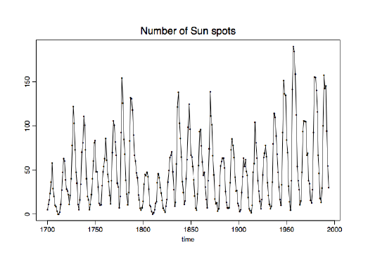
Example 1.1.1 (W\(\ddot{\mbox{o}}\)lfer's sunspot numbers). In Figure 1.1, the number of sunspots (that is, dark spots visible on the surface of the sun) observed annually are plotted against time. The horizontal axis labels time in years, while the vertical axis represents the observed values \(x_t\) of the random variable
\[ X_t=\#\mbox{ of sunspots at time $t$},\qquad t=1700,\ldots,1994. \nonumber \]
The figure is called a time series plot. It is a useful device for a preliminary analysis. Sunspot numbers are used to explain magnetic oscillations on the sun surface.

Figure 1.1: Wölfer's sunspot from 1700 to 1994.
To reproduce a version of the time series plot in Figure 1.1 using the free software package R (downloads are available at http://cran.r-project.org), download the file sunspots.dat from the course webpage and type the following commands:
> spots = read.table("sunspots.dat")
> spots = ts(spots, start=1700, frequency=1)
> plot(spots, xlab="time", ylab="", main="Number of Sun spots")
In the first line, the file sunspots.dat is read into the object spots, which is then in the second line transformed into a time series object using the function ts(). Using start sets the starting value for the x-axis to a prespecified number, while frequency presets the number of observations for one unit of time. (Here: one annual observation.) Finally, plot is the standard plotting command in R, where xlab and ylab determine the labels for the x-axis and y-axis, respectively, and main gives the headline.
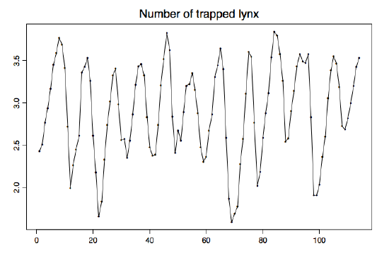
Example 1.1.2 (Canadian lynx data). The time series plot in Figure 1.2 comes from a biological data set. It contains the annual returns of lynx at auction in London by the Hudson Bay Company from 1821--1934 (on a \(log_{10}\) scale). These are viewed as observations of the stochastic process
\[ X_t=\log_{10}(\mbox{number of lynx trapped at time $1820+t$}), \qquad t=1,\ldots,114. \nonumber \]

Figure 1.2: Number of lynx trapped in the MacKenzie River district between 1821 and 1934.
The data is used as an estimate for the number of all lynx trapped along the MacKenzie River in Canada. This estimate, in turn, is often taken as a proxy for the true population size of the lynx. A similar time series plot could be obtained for the snowshoe rabbit, the primary food source of the Canadian lynx, hinting at an intricate predator-prey relationship.
Assuming that the data is stored in the file lynx.dat, the corresponding R commands leading to the time series plot in Figure 1.2 are:
> lynx = read.table("lynx.dat")
> lynx = ts(log10(lynx), start=1821, frequency=1)
> plot(lynx, xlab="", ylab="", main="Number of trapped lynx")
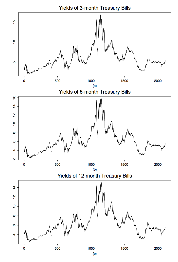
Example 1.1.3 (Treasury bills). Another important field of application for time series analysis lies in the area of finance. To hedge the risks of portfolios, investors commonly use short-term risk-free interest rates such as the yields of three-month, six-month, and twelve-month Treasury bills plotted in Figure 1.3. The (multivariate) data displayed consists of 2,386 weekly observations from July 17, 1959, to December 31, 1999. Here,
\[ X_t=(X_{t,1},X_{t,2},X_{t,3}), \qquad t=1,\ldots,2386, \nonumber \]
where \(X_{t,1}\), \(X_{t,2}\) and \(X_{t,3}\) denote the three-month, six-month, and twelve-month yields at time t, respectively. It can be seen from the graph that all three Treasury bills are moving very similarly over time, implying a high correlation between the components of \(X_t\).

Figure 1.3: Yields of Treasury bills from July 17, 1959, to December 31, 1999.

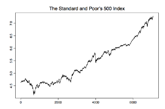
Figure 1.4: S&P 500 from January 3, 1972, to December 31, 1999.
To produce the three-variate time series plot in Figure 1.3, use the R code
> bills03 = read.table("bills03.dat");
> bills06 = read.table("bills06.dat");
> bills12 = read.table("bills12.dat");
> par(mfrow=c(3,1))
> plot.ts(bills03, xlab="(a)", ylab="",
main="Yields of 3-month Treasury Bills")
> plot.ts(bills06, xlab="(b)", ylab="",
main="Yields of 6-month Treasury Bills")
> plot.ts(bills12, xlab="(c)", ylab="",
main="Yields of 12-month Treasury Bills")
It is again assumed that the data can be found in the corresponding files bills03.dat, bills06.dat and bills12.dat. The command line par(mfrow=c(3,1)) is used to set up the graphics. It enables you to save three different plots in the same file.
Example 1.1.4 (S&P 500). The Standard and Poor's 500 index (S&P 500) is a value-weighted index based on the prices of 500 stocks that account for approximately 70% of the U.S. equity market capitalization. It is a leading economic indicator and is also used to hedge market portfolios. Figure 1.4 contains the 7,076 daily S&P 500 closing prices from January 3, 1972, to December 31, 1999, on a natural logarithm scale. It is consequently the time series plot of the process
\[ X_t=\ln(\mbox{closing price of S&P 500 at time $t$}), \qquad t=1,\ldots,7076. \nonumber \]
Note that the logarithm transform has been applied to make the returns directly comparable to the percentage of investment return. The time series plot can be reproduced in R using the file sp500.dat
There are countless other examples from all areas of science. To develop a theory capable of handling broad applications, the statistician needs to rely on a mathematical framework that can explain phenomena such as
- trends (apparent in Example 1.1.4);
- seasonal or cyclical effects (apparent in Examples 1.1.1 and 1.1.2);
- random fluctuations (all Examples);
- dependence (all Examples?).
The classical approach taken in time series analysis is to postulate that the stochastic process \((X_t\colon t\in T)\) under investigation can be divided into deterministic trend and seasonal components plus a centered random component, giving rise to the model
\[X_t=m_t+s_t+Y_t, \qquad t\in T \tag{1.1.1} \]
where \((m_t\colon t\in T)\) denotes the trend function ("mean component''), \((s_t\colon t\in T)\) the seasonal effects and \((Y_t\colon t\in T)\) a (zero mean) stochastic process. After an appropriate model has been chosen, the statistician may aim at
- estimating the model parameters for a better understanding of the time series;
- predicting future values, for example, to develop investing strategies;
- checking the goodness of fit to the data to confirm that the chosen model is appropriate.
Estimation procedures and prediction techniques are dealt with in detail in later chapters of the notes. The rest of this chapter will be devoted to introducing the classes of strictly and weakly stationary stochastic processes (in Section 1.2) and to providing tools to eliminate trends and seasonal components from a given time series (in Sections 1.3 and 1.4), while some goodness of fit tests will be presented in Section 1.5.


