9.3: Ants learn to rely on more informative attributes during decision-making

In Sasaki and Pratt (2013), a set of ant colonies were randomly assigned to one of two treatments to study whether the ants could be “trained” to have a preference for or against certain attributes for potential nest sites. The colonies were either randomly assigned to experience the repeated choice of two identical colony sites except for having an inferior light or entrance size attribute. Then the ants were allowed to choose between two nests, one that had a large entrance but was dark and the other that had a small entrance but was bright. 54 of the 60 colonies that were randomly assigned to one of the two treatments completed the experiment by making a choice between the two types of sites. The data set and some processing code follows.

The first question is what type of analysis is appropriate here. Once we recognize that there are two categorical variables being considered (Treatment group with two levels and After choice with two levels SmallBright or LargeDark for what the colonies selected), then this is recognized as being within our Chi-square testing framework. The random assignment of colonies (the subjects here) to treatment levels tells us that the Chi-square Homogeneity test is appropriate here and that we can make causal statements about the effects of the Treatment groups.

sasakipratt <- read_csv("http://www.math.montana.edu/courses/s217/documents/sasakipratt.csv")

sasakipratt <- sasakipratt %>% mutate(group = factor(group),
                                      after = factor(after),
                                      before = factor(before)
                                      )
levels(sasakipratt$group) <- c("Light", "Entrance")
levels(sasakipratt$after) <- c("SmallBright", "LargeDark")
levels(sasakipratt$before) <- c("SmallBright", "LargeDark")
plot(after ~ group, data = sasakipratt, col = cividis(2))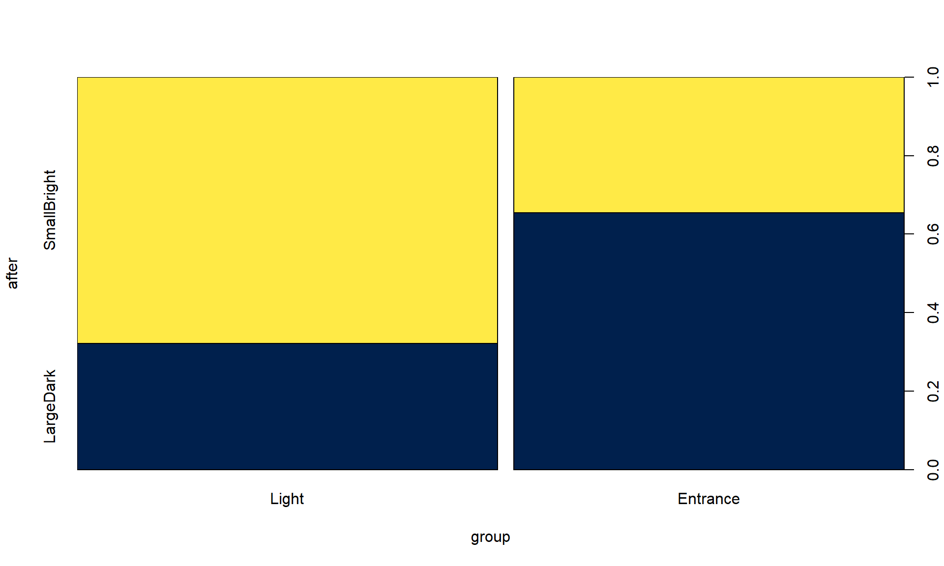

Figure 9.9: Stacked bar chart for Ant Colony results.

library(mosaic)
tally(~ group + after, data = sasakipratt)

##           after
## group      SmallBright LargeDark
##   Light             19         9
##   Entrance           9        17

table1 <- tally(~ group + after, data = sasakipratt, margins = F)

The null hypothesis of interest here is that there is no difference in the distribution of responses on After – the rates of their choice of den types – between the two treatment groups in the population of all ant colonies like those studied. The alternative is that there is some difference in the distributions of After between the groups in the population.

To use the Chi-square distribution to find a p-value for the \(X^2\) statistic, we need all the expected cell counts to be larger than 5, so we should check that. Note that in the following, the correct = F option is used to keep the function from slightly modifying the statistic used that occurs when overall sample sizes are small.

chisq.test(table1, correct = F)$expected

##           after
## group      SmallBright LargeDark
##   Light       14.51852  13.48148
##   Entrance    13.48148  12.51852

Our expected cell count condition is met, so we can proceed to explore the results of the parametric test:

chisq.test(table1, correct = F)

## 
##  Pearson's Chi-squared test
## 
## data:  table1
## X-squared = 5.9671, df = 1, p-value = 0.01458

The \(X^2\) statistic is 5.97 which, if our assumptions hold, should approximately follow a Chi-square distribution with \((R-1)*(C-1) = 1\) degrees of freedom under the null hypothesis. The p-value is 0.015, suggesting that there is moderate to strong evidence against the null hypothesis and we can conclude that there is a difference in the distribution of the responses between the two treated groups in the population of all ant colonies that could have been treated. Because of the random assignment, we can say that the treatments caused differences in the colony choices. These results cannot be extended to ants beyond those being studied by these researchers because they were not randomly selected.

Further exploration of the standardized residuals can provide more insights in some situations, although here they are similar for all the cells:

chisq.test(table1, correct = F)$residuals

##           after
## group      SmallBright LargeDark
##   Light       1.176144 -1.220542
##   Entrance   -1.220542  1.266616

When all the standardized residual contributions are similar, that suggests that there are differences in all the cells from what we would expect if the null hypothesis were true. Basically, that means that what we observed is a bit larger than expected for the Light treatment group in the SmallBright choice and lower than expected in LargeDark – those treated ants preferred the small and bright den. And for the Entrance treated group, they preferred the large entrance, dark den at a higher rate than expected if the null is true and lower than expected in the small entrance, bright location.

The researchers extended this basic result a little further using a statistical model called logistic regression, which involves using something like a linear model but with a categorical response variable (well – it actually only works for a two-category response variable). They also had measured which of the two types of dens that each colony chose before treatment and used this model to control for that choice. So the actual model used in their paper contained two predictor variables – the randomized treatment received that we explored here and the prior choice of den type. The interpretation of their results related to the same treatment effect, but they were able to discuss it after adjusting for the colonies previous selection. Their conclusions were similar to those found with our simpler analysis. Logistic regression models are a special case of what are called generalized linear models and are a topic for the next level of statistics if you continue exploring.