4.3: Two-Way ANOVA models and hypothesis tests

To assess interactions with two variables, we need to fully describe models for the additive and interaction scenarios and then develop a method for assessing evidence of the need for different aspects of the models. First, we need to define the notation for these models:

• \(y_{ijk}\) is the \(i^{th}\) response from the group for level \(j\) of factor A and level \(k\) of factor B
  • \(j = 1,\ldots,J\) \(J\) is the number of levels of A
  • \(k = 1,\ldots,K\) \(K\) is the number of levels of B
  • \(i = 1,\ldots,n_{jk}\) \(n_{jk}\) is the sample size for level \(j\) of factor A and level \(k\) of factor B
  • \(N = \Sigma_j\Sigma_k n_{jk}\) is the total sample size (sum of the number of observations across all \(JK\) groups)

We need to extend our previous discussion of reference-coded models to develop a Two-Way ANOVA model. We start with the Two-Way ANOVA interaction model:

\[y_{ijk} = \alpha + \tau_j + \gamma_k + \omega_{jk} + \varepsilon_{ijk},\]

where \(\alpha\) is the baseline group mean (for level 1 of A and level 1 of B), \(\tau_j\) is the deviation for the main effect of A from the baseline for levels \(2,\ldots,J\), \(\gamma_k\) (gamma \(k\)) is the deviation for the main effect of B from the baseline for levels \(2,\ldots,K\), and \(\omega_{jk}\) (omega \(jk\)) is the adjustment for the interaction effect for level \(j\) of factor A and level \(k\) of factor B for \(j = 1,\ldots,J\) and \(k = 1,\ldots,K\). In this model, \(\tau_1\), \(\gamma_1\), and \(\omega_{11}\) are all fixed at 0 because \(\alpha\) is the mean for the combination of the baseline levels of both variables and so no adjustments are needed. Additionally, any \(\omega_{jk}\)’s that contain the baseline category of either factor A or B are also set to 0 and the model for these levels just involves \(\tau_j\) or \(\gamma_k\) added to the intercept. Exploring the R output will help clarify which coefficients are present or set to 0 (so not displayed) in these models. As in Chapter 3, R will typically choose the baseline categories alphabetically but now it is choosing a baseline for both variables and so our detective work will be doubled to sort this out.

If the interaction term is not important, usually based on the interaction test presented below, the \(\omega_{jk}\text{'s}\) can be dropped from the model and we get a model that corresponds to Scenario 4 above. Scenario 4 is where there are two main effects in the model but no interaction between them. The additive Two-Way model is

\[y_{ijk} = \alpha + \tau_j + \gamma_k + \varepsilon_{ijk},\]

where each component is defined as in the interaction model. The difference between the interaction and additive models is setting all the \(\omega_{jk}\text{'s}\) to 0 that are present in the interaction model. When we set parameters to 0 in models it removes them from the model. Setting parameters to 0 is also how we will develop our hypotheses to test for an interaction, by assessing evidence against a null hypothesis that all \(\omega_{jk}\text{'s} = 0\).

The interaction test hypotheses are

• \(H_0\): No interaction between A and B on response in population \(\Leftrightarrow\) All \(\omega_{jk}\text{'s} = 0\).
• \(H_A\): Interaction between A and B on response in population \(\Leftrightarrow\) At least one \(\omega_{jk}\ne 0\).

To perform this test, a new ANOVA \(F\)-test is required (presented below) but there are also hypotheses relating to the main effects of A (\(\tau_j\text{'s}\)) and B (\(\gamma_k\text{'s}\)). If you decide that there is sufficient evidence against the null hypothesis that no interaction is present to conclude that one is likely present, then it is dangerous to ignore the interaction and test for the main effects because important main effects can be masked by interactions (examples later). It is important to note that, by definition, both variables matter if an interaction is found to be important so the main effect tests may not be very interesting in an interaction model. If the interaction is found to be important based on the test and so is retained in the model, you should focus on the interaction model (also called the full model) in order to understand and describe the form of the interaction among the variables.

If the interaction test does not return a small p-value and you decide that you do not have enough evidence against the null hypothesis to suggest that the interaction is needed, the interaction can be dropped from the model. In this situation, we would re-fit the model and focus on the results provided by the additive model – performing tests for the two additive main effects. For the first, but not last time, we encounter a model with more than one variable and more than one test of potential interest. In models with multiple variables at similar levels (here both are main effects), we are interested in the results for each variable given that the other variable is in the model. In many situations, including more than one variable in a model changes the results for the other variable even if those variables do not interact. The reason for this is more clear in Chapter 8 and really only matters here if we have unbalanced designs, but we need to start adding a short modifier to our discussions of main effects – they are the results conditional on or adjusting for or, simply, given, the other variable(s) in the model. Specifically, the hypotheses for the two main effects are:

• Main effect test for A:
  • \(H_0\): No differences in means across levels of A in population, given B in the model

    \(\Leftrightarrow\) All \(\tau_j\text{'s} = 0\) in additive model.

  • \(H_A\): Some difference in means across levels A in population, given B in the model

    \(\Leftrightarrow\) At least one \(\tau_j \ne 0\), in additive model.

• Main effect test for B:
  • \(H_0\): No differences in means across levels of B in population, given A in the model

    \(\Leftrightarrow\) All \(\gamma_k\text{'s} = 0\) in additive model.

  • \(H_A\): Some difference in means across levels B in population, given A in the model

    \(\Leftrightarrow\) At least one \(\gamma_k \ne 0\), in additive model.

In order to test these effects (interaction in the interaction model and main effects in the additive model), \(F\)-tests are developed using Sums of Squares, Mean Squares, and degrees of freedom similar to those in Chapter 3. We won’t worry about the details of the sums of squares formulas but you should remember the sums of squares decomposition, which still applies⁸⁴. Table 4.1 summarizes the ANOVA results you will obtain for the interaction model and Table 4.2 provides the similar general results for the additive model. As we saw in Chapter 3, the degrees of freedom are the amount of information that is free to vary at a particular level and that rule generally holds here. For example, for factor A with \(J\) levels, there are \(J-1\) parameters that are free since the baseline is fixed. The residual degrees of freedom for both models are not as easily explained but have a simple formula. Note that the sum of the degrees of freedom from the main effects, (interaction if present), and error need to equal \(N-1\), just like in the One-Way ANOVA table.

Table 4.1: Interaction Model ANOVA Table.

Source	DF	SS	MS	F-statistics
A	\(J-1\)	\(\text{SS}_A\)	\(\text{MS}_A = \text{SS}_A/\text{df}_A\)	\(\text{MS}_A/\text{MS}_E\)
B	\(K-1\)	\(\text{SS}_B\)	\(\text{MS}_B = \text{SS}_B/\text{df}_B\)	\(\text{MS}_B/\text{MS}_E\)
A:B (interaction)	\((J-1)(K-1)\)	\(\text{SS}_{AB}\)	\(\text{MS}_{AB} = \text{SS}_{AB}/\text{df}_{AB}\)	\(\text{MS}_{AB}/\text{MS}_E\)
Error	\(N-JK\)	\(\text{SS}_E\)	\(\text{MS}_E = \text{SS}_E/\text{df}_E\)
Total	\(\color{red}{\mathbf{N-1}}\)	\(\color{red}{\textbf{SS}_{\textbf{Total}}}\)

Table 4.2: Additive Model ANOVA Table.

Source	DF	SS	MS	F-statistics
A	\(J-1\)	\(\text{SS}_A\)	\(\text{MS}_A = \text{SS}_A/\text{df}_A\)	\(\text{MS}_A/\text{MS}_E\)
B	\(K-1\)	\(\text{SS}_B\)	\(\text{MS}_B = \text{SS}_B/\text{df}_B\)	\(\text{MS}_B/\text{MS}_E\)
Error	\(N-J-K+1\)	\(\text{SS}_E\)	\(\text{MS}_E = \text{SS}_E/\text{df}_E\)
Total	\(\color{red}{\mathbf{N-1}}\)	\(\color{red}{\textbf{SS}_{\textbf{Total}}}\)

The mean squares are formed by taking the sums of squares (we’ll let R find those for us) and dividing by the \(df\) in the row. The \(F\)-ratios are found by taking the mean squares from the row and dividing by the mean squared error (\(\text{MS}_E\)). They follow \(F\)-distributions with numerator degrees of freedom from the row and denominator degrees of freedom from the Error row (in R output this the Residuals row). It is possible to develop permutation tests for these methods but some technical issues arise in doing permutation tests for interaction model components so we will not use them here. This means we will have to place even more emphasis on the data not presenting clear violations of assumptions since we only have the parametric method available.

With some basic expectations about the ANOVA tables and \(F\)-statistic construction in mind, we can get to actually estimating the models and exploring the results. The first example involves the fake paper towel data displayed in Figure 4.1 and 4.2. It appeared that Scenario 5 was the correct story since the lines appeared to be non-parallel, but we need to know whether there is sufficient evidence to suggest that the interaction is “real” and we get that through the interaction hypothesis test. To fit the interaction model using lm, the general formulation is lm(y ~ x1 * x2, data = ...). The order of the variables doesn’t matter as the most important part of the model, to start with, relates to the interaction of the variables.

The ANOVA table output shows the results for the interaction model obtained by running the anova function on the model called m1. Specifically, the test that \(H_0: \text{ All } \omega_{jk}\text{'s} = 0\) has a test statistic of \(F(2,24) = 1.92\) (in the output from the row with brands:drops) and a p-value of 0.17. So there is weak evidence against the null hypothesis of no interaction, with a 17% chance we would observe a difference in the \(\omega_{jk}\text{'s}\) like we did or more extreme if the \(\omega_{jk}\text{'s}\) really were all 0. So we would conclude that the interaction is probably not needed⁸⁵. Note that for the interaction model components, R presents them with a colon, :, between the variable names.

m1 <- lm(responses ~ brand * drops, data = pt)
anova(m1)

## Analysis of Variance Table
## 
## Response: responses
##             Df Sum Sq Mean Sq F value   Pr(>F)
## brand        1 4.3322  4.3322 10.5192 0.003458
## drops        2 4.8581  2.4290  5.8981 0.008251
## brand:drops  2 1.5801  0.7901  1.9184 0.168695
## Residuals   24 9.8840  0.4118

It is useful to display the estimates from this model and we can utilize plot(allEffects(MODELNAME)) to visualize the results for the terms in our models. If we turn on the options for grid = T, multiline = T, and ci.style = "bars" we get a useful version of the basic “effect plot” for Two-Way ANOVA models with interaction. I also added lty = c(1:2) to change the line type for the two lines (replace 2 with the number of levels in the variable driving the different lines. The results of the estimated interaction model are displayed in Figure 4.7, which looks very similar to our previous interaction plot. The only difference is that this comes from model that assumes equal variance and these plots show 95% confidence intervals for the means instead of the \(\pm\) 1 SE used in the intplot where each SE is calculated using the variance of the observations at each combination of levels. Note that other than the lines connecting the means, this plot also is similar to the pirate-plot in Figure 4.1 that also displayed the original responses for each of the six combinations of the two explanatory variables. That plot then provides a place to assess assumptions of the equal variance and distributions for each group as well as explore differences in the group means.

library(effects)
plot(allEffects(m1), grid = T, multiline = T, lty = c(1:2), ci.style = "bars")

Figure 4.7: Plot of estimated results of interaction model for the paper towel performance data.

In the absence of sufficient evidence to include the interaction, the model should be simplified to the additive model and the interpretation focused on each main effect, conditional on having the other variable in the model. To fit an additive model and not include an interaction, the model formula involves a “+” instead of a “*” between the explanatory variables.

m2 <- lm(responses ~ brand + drops, data = pt)
anova(m2)

## Analysis of Variance Table
## 
## Response: responses
##           Df  Sum Sq Mean Sq F value   Pr(>F)
## brand      1  4.3322  4.3322  9.8251 0.004236
## drops      2  4.8581  2.4290  5.5089 0.010123
## Residuals 26 11.4641  0.4409

The p-values for the main effects of brand and drops change slightly from the results in the interaction model due to changes in the \(\text{MS}_E\) from 0.4118 to 0.4409 (more variability is left over in the simpler model) and the \(\text{DF}_{\text{error}}\) that increases from 24 to 26. In both models, the \(\text{SS}_{\text{Total}}\) is the same (20.6544). In the interaction model,

\[\begin{array}{rl} \text{SS}_{\text{Total}} & = \text{SS}_{\text{brand}} + \text{SS}_{\text{drops}} + \text{SS}_{\text{brand:drops}} + \text{SS}_{\text{E}}\\ & = 4.3322 + 4.8581 + 1.5801 + 9.8840\\ & = 20.6544.\\ \end{array}\]

In the additive model, the variability that was attributed to the interaction term in the interaction model (\(\text{SS}_{\text{brand:drops}} = 1.5801\)) is pushed into the \(\text{SS}_{\text{E}}\), which increases from 9.884 to 11.4641. The sums of squares decomposition in the additive model is

\[\begin{array}{rl} \text{SS}_{\text{Total}} & = \text{SS}_{\text{brand}} + \text{SS}_{\text{drops}} + \text{SS}_{\text{E}} \\ & = 4.3322 + 4.8581 + 11.4641 \\ & = 20.6544. \\ \end{array}\]

This shows that the sums of squares decomposition applies in these more complicated models as it did in the One-Way ANOVA. It also shows that if the interaction is removed from the model, that variability is lumped in with the other unexplained variability that goes in the \(\text{SS}_{\text{E}}\) in any model.

The fact that the sums of squares decomposition can be applied here is useful, except that there is a small issue with the main effect tests in the ANOVA table results that follow this decomposition when the design is not balanced. It ends up that the tests in a typical ANOVA table are only conditional on the tests higher up in the table. For example, in the additive model ANOVA table, the Brand test is not conditional on the Drops effect, but the Drops effect is conditional on the Brand effect. In balanced designs, conditioning on the other variable does not change the results but in unbalanced designs, the order does matter. To get both results to be similarly conditional on the other variable, we have to use another type of sums of squares, called Type II sums of squares. These sums of squares will no longer always follow the rules of the sums of squares decomposition but they will test the desired hypotheses. Specifically, they provide each test conditional on any other terms at the same level of the model and match the hypotheses written out earlier in this section. To get the “correct” ANOVA results, the car package (Fox, Weisberg, and Price (2022a), Fox and Weisberg (2011)) is required. We use the Anova function on our linear models from here forward to get the “right” tests in our ANOVA tables⁸⁶. Note how the case-sensitive nature of R code shows up in the use of the capital “A” Anova function instead of the lower-case “a” anova function used previously. In this situation, because the design was balanced, the results are the same using either function. Observational studies rarely generate balanced designs (some designed studies can result in unbalanced designs too) so we will generally just use the Type II version of the sums of squares to give us the desired results across different data sets we might analyze. The Anova results using the Type II sums of squares are slightly more conservative than the results from anova, which are called Type I sums of squares. The sums of squares decomposition no longer applies, but it is a small sacrifice to get each test after adjusting for all other variables⁸⁷.

library(car)
Anova(m2)

## Anova Table (Type II tests)
## 
## Response: responses
##            Sum Sq Df F value   Pr(>F)
## brand      4.3322  1  9.8251 0.004236
## drops      4.8581  2  5.5089 0.010123
## Residuals 11.4641 26

The new output switches the columns around and doesn’t show you the mean squares, but gives the most critical parts of the output. Here, there is no change in results because it is a balanced design with equal counts of responses in each combination of the two explanatory variables.

The additive model, when appropriate, provides simpler interpretations for each explanatory variable compared to models with interactions because the effect of one variable is the same regardless of the levels of the other variable and vice versa. There are two tools to aid in understanding the impacts of the two variables in the additive model. First, the model summary provides estimated coefficients with interpretations like those seen in Chapter 3 (deviation of group \(j\) or \(k\) from the baseline group’s mean), except with the additional wording of “controlling for” the other variable added to any of the discussion. Second, the term-plots now show each main effect and how the groups differ with one panel for each of the two explanatory variables in the model. These term-plots are created by holding the other variable constant at one of its levels (the most frequently occurring or first if the there are multiple groups tied for being most frequent) and presenting the estimated means across the levels of the variable in the plot.

summary(m2)

## 
## Call:
## lm(formula = responses ~ brand + drops, data = pt)
## 
## Residuals:
##     Min      1Q  Median      3Q     Max 
## -1.4561 -0.4587  0.1297  0.4434  0.9695 
## 
## Coefficients:
##             Estimate Std. Error t value Pr(>|t|)
## (Intercept)   1.8454     0.2425   7.611 4.45e-08
## brandB2       0.7600     0.2425   3.134  0.00424
## drops20      -0.4680     0.2970  -1.576  0.12715
## drops30      -0.9853     0.2970  -3.318  0.00269
## 
## Residual standard error: 0.664 on 26 degrees of freedom
## Multiple R-squared:  0.445,  Adjusted R-squared:  0.3809 
## F-statistic: 6.948 on 3 and 26 DF,  p-value: 0.001381

In the model summary, the baseline combination estimated in the (Intercept) row is for Brand B1 and Drops 10 and estimates the mean failure time as 1.85 seconds for this combination. As before, the group labels that do not show up are the baseline but there are two variables’ baselines to identify. Now the “simple” aspects of the additive model show up. The interpretation of the Brands B2 coefficient is as a deviation from the baseline but it applies regardless of the level of Drops. Any difference between B1 and B2 involves a shift up of 0.76 seconds in the estimated mean failure time. Similarly, going from 10 (baseline) to 20 drops results in a drop in the estimated failure mean of 0.47 seconds and going from 10 to 30 drops results in a drop of almost 1 second in the average time to failure, both estimated changes are the same regardless of the brand of paper towel being considered. Sometimes, especially in observational studies, we use the terminology “controlled for” to remind the reader that the other variable was present in the model⁸⁸ and also explained some of the variability in the responses. The term-plots for the additive model (Figure 4.8) help us visualize the impacts of changes brand and changing water levels, holding the other variable constant. The differences in heights in each panel correspond to the coefficients just discussed.

library(effects)
plot(allEffects(m2))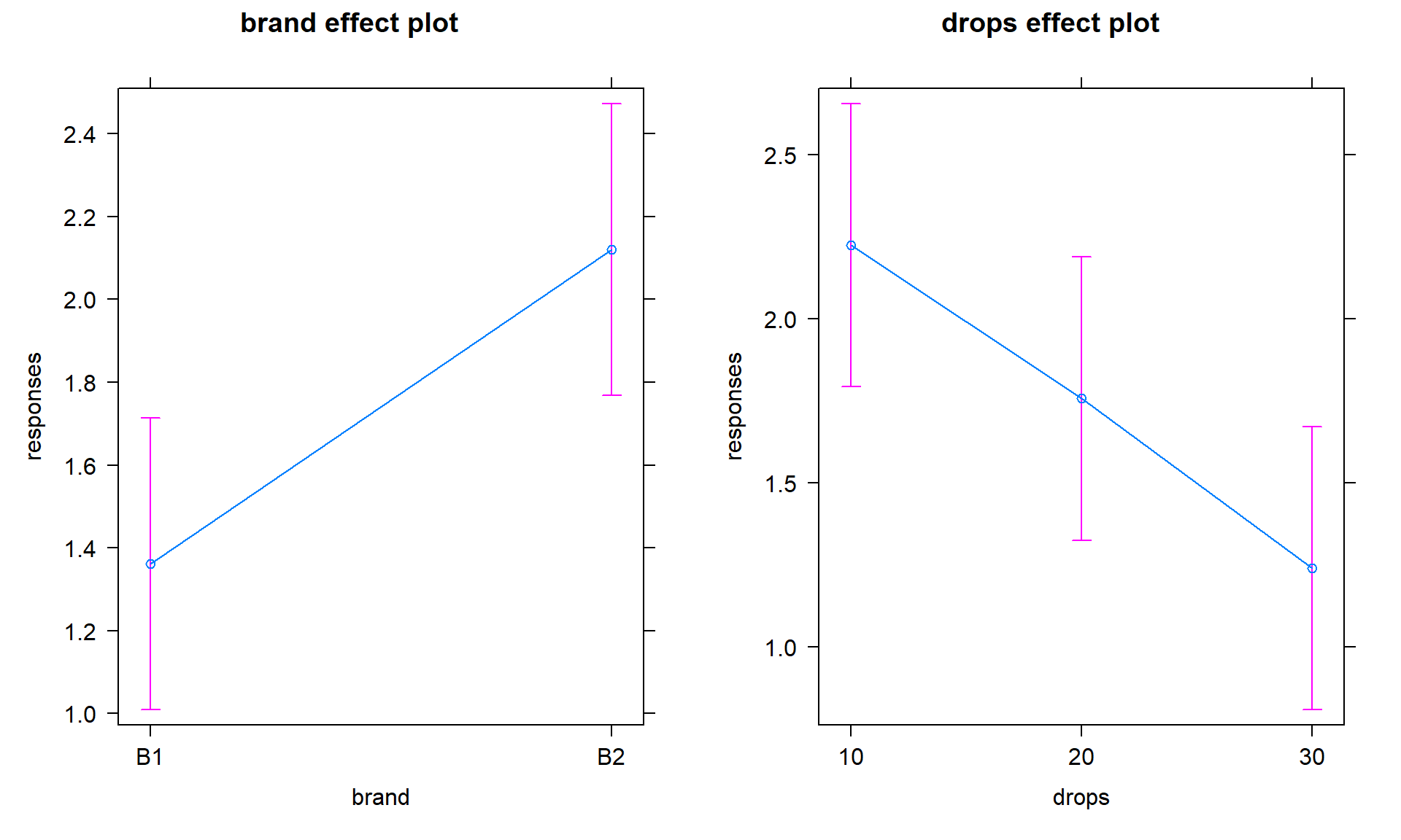

Figure 4.8: Term-plots of additive model for paper towel data. Left panel displays results for two brands and right panel for number of drops of water, each after controlling for the other.

With the first additive model we have considered, it is now the first time where we are working with a model where we can’t display the observations together with the means that the model is producing because the results for each predictor are averaged across the levels of the other predictor. To visualize some aspects of the original observations with the estimates from each group, we can turn on an option in the term-plots (residuals = T) to obtain the partial residuals that show the residuals as a function of one variable after adjusting for the effects/impacts of other variables. We will avoid the specifics of the calculations for now, but you can use these to explore the residuals at different levels of each predictor. They will be most useful in the Chapters 7 and 8 but give us some insights in unexplained variation in each level of the predictors once we remove the impacts of other predictors in the model. Use plots like Figure 4.9 to look for different variability at different levels of the predictors and locations of possible outliers in these models. Note that the points (open circles) are jittered to aid in seeing all of them, the means of each group of residuals are indicated by a filled large circle, and the smaller circles in the center of the bars for the 95% confidence intervals are the means from the model. Term-plots with partial residuals accompany our regular diagnostic plots for assessing equal variance assumptions in these models – in some cases adding the residuals will clutter the term-plots so much that reporting them is not useful since one of the main purposes of the term-plots is to visualize the model estimates. So use the residuals = T option judiciously.

library(effects)
plot(allEffects(m2, residuals = T))

Figure 4.9: Term-plots of additive model for paper towel data with partial residuals added. Relatively similar variability seems to be present in each of the groups of residuals after adjusting for the other variable except for the residuals for the 10 drops where the variability is smaller, especially if one small outlier is ignored.

For the One-Way and Two-Way interaction models, the partial residuals are just the original observations so present similar information as the pirate-plots but do show the model estimated 95% confidence intervals. With interaction models, you can use the default settings in effects when adding in the partial residuals as seen below in Figure 4.12.