
9.4: Using Technology - Equal Slopes Model
- Page ID
- 33169

Using Technology
Using our Salary example using the data in the table below, we can run through the steps for the ANCOVA.
| Females | Males | ||
|---|---|---|---|
| Salary | Years | Salary | Years |
| 80 | 5 | 78 | 3 |
| 50 | 3 | 43 | 1 |
| 30 | 2 | 103 | 5 |
| 20 | 1 | 48 | 2 |
| 60 | 4 | 80 | 4 |
- Steps in SAS
-
Step 1: Are all regression slopes = 0?
A simple linear regression can be run for each treatment group, Males and Females.
Running these procedures using statistical software we get the following:
Males
Use the following SAS code:
data equal_slopes;
input gender $ salary years;
datalines;
m 78 3
m 43 1
m 103 5
m 48 2
m 80 4
f 80 5
f 50 3
f 30 2
f 20 1
f 60 4
;
proc reg data=equal_slopes;
where gender='m';
model salary=years;
title 'Males';
run; quit;
And here is the output that you get:
The REG Procedure
Mode1:: MODEL1
Dependent Variable: salaryNumber of Observations Read 5 Number of Observations Used 5 Analysis of Variance Source DF Sum of Squares Mean Square F Value Pr > F Model 1 2310.40000 2310.40000 44.78 F" class=" ">0.0068 Error 3 154.80000 51.60000 F" class=" "> Corrected Total 4 2465.20000 Females
Use the following SAS code:
data equal_slopes;
input gender $ salary years;
datalines;
m 78 3
m 43 1
m 103 5
m 48 2
m 80 4
f 80 5
f 50 3
f 30 2
f 20 1
f 60 4
;
proc reg data=equal_slopes;
where gender='f';
model salary=years;
title 'Females';
run; quit;
And here is the output for this run:
The REG Procedure
Mode1:: MODEL1
Dependent Variable: salaryNumber of Observations Read 5 Number of Observations Used 5 Analysis of Variance Source DF Sum of Squares Mean Square F Value Pr > F Model 1 2250.00000 2250.00000 225.00 F" class=" ">0.0006 Error 3 30.00000 10.00000 F" class=" "> Corrected Total 4 2280.00000 F" class=" "> In both cases, the simple linear regressions are significant, so the slopes are not = 0.
Step 2: Are the slopes equal?
We can test for this using our statistical software.
In SAS we now use proc mixed and include the covariate in the model.
We will also include a "treatment × covariate" interaction term and the significance of this term answers our question. If the slopes differ significantly among treatment levels, the interaction \(p\)-value will be < 0.05.
If the slopes differ significantly among treatment levels, the interaction p-value will be < 0.05.
data equal_slopes;
input gender $ salary years;
datalines;
m 78 3
m 43 1
m 103 5
m 48 2
m 80 4
f 80 5
f 50 3
f 30 2
f 20 1
f 60 4
;
proc mixed data=equal_slopes;
class gender;
model salary = gender years gender*years;
run;
In SAS, we specify the treatment in the class statement, indicating that these are categorical levels. By NOT including the covariate in the class statement, it will be treated as a continuous variable for regression in the model statement.
The Mixed Procedure
Type 3 Tests of Fixed EffectsEffect Num DF Den DF F Value Pr > F years 1 6 148.06 F" class=" "><.0001 gender 1 6 7.01 F" class=" ">0.0381 years*gender 1 6 0.01 F" class=" ">0.9384 So here we see that the slopes are equal and in a plot of the regressions, we see that the lines are parallel.
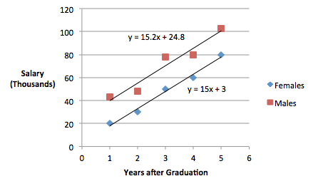
Figure \(\PageIndex{a1}\): Parallel lines of best fit To obtain the plot in SAS, we can use the following SAS code:
SAS code:
ods graphics on;
proc sgplot data=equal_slopes;
styleattrs datalinepatterns=(solid);
reg y=salary x=years / group=gender;
run;
Step 3: Fit an Equal Slopes Model
We can now proceed to fit an Equal Slopes model by removing the interaction term. Again, we will use our statistical software SAS.
data equal_slopes;
input gender $ salary years;
datalines;
m 78 3
m 43 1
m 103 5
m 48 2
m 80 4
f 80 5
f 50 3
f 30 2
f 20 1
f 60 4
;
proc mixed data=equal_slopes;
class gender;
model salary = gender years;
lsmeans gender / pdiff adjust=tukey;
/* Tukey unnecessary with only two treatment levels */
title 'Equal Slopes Model';
run;
We obtain the following results:
The Mixed Procedure
Type 3 Tests of Fixed EffectsEffect Num DF Den DF F Value Pr > F years 1 7 172.55 F" class=" "><.0001 gender 1 7 47.46 F" class=" ">0.0002 Least Squares Means Effect gender Estimate Standard Error DF t Value Pr > |t| gender f 48.0000 2.2991 7 20.88 |t|" class=" "><.0001 gender m 70.4000 2.2991 7 30.62 |t|" class=" "><.0001 In SAS, the model statement automatically creates an intercept, and so the ANCOVA model is technically over-parameterized. To get the slopes and intercepts for the covariate directly, we have to re-parameterize the model. This entails suppressing the intercept ( noint ), and then specifying that we want the solutions, ( solution ), to the model. Here is what the SAS code looks like for this:
data equal_slopes;
input gender $ salary years;
datalines;
m 78 3
m 43 1
m 103 5
m 48 2
m 80 4
f 80 5
f 50 3
f 30 2
f 20 1
f 60 4
;
proc mixed data=equal_slopes;
class gender;
model salary = gender years / noint solution;
ods select SolutionF;
title 'Equal Slopes Model';
run;
Here is the output:
Solution for Fixed Effects Effect gender Estimate Standard Error DF t Value Pr > |t| gender f 2.7000 4.1447 7 0.65 |t|" class=" ">0.5356 gender m 25.1000 4.1447 7 6.06 |t|" class=" ">0.0005 years 15.1000 1.1495 7 13.14 |t|" class=" "><.0001 In the first section of the output above is reported a separate intercept for each gender, the ‘Estimate’ value for each gender, and a common slope for both genders, labeled ‘Years’.
Thus, the estimated regression equation for Females is \(\hat{y} = 2.7 + 15.1(\text{Years})\), and for Males it is \(\hat{y} = 25.1 _ 15.1(\text{Years})\).
To this point in this analysis, we can see that 'gender' is now significant. By removing the impact of the covariate, we went from
Type 3 Tests of Fixed Effects Effect Num DF Den DF F Value Pr > F gender 1 8 2.11 F" class=" ">0.1840 (without covariate consideration)
to
gender 1 7 47.46 0.0002 (adjusting for the covariate)
Using our Salary example and the data in the table below, we can run through the steps for the ANCOVA. On this page, we will go through the steps using Minitab.
| Females | Males | ||
|---|---|---|---|
| Salary | Years | Salary | Years |
| 80 | 5 | 78 | 3 |
| 50 | 3 | 43 | 1 |
| 30 | 2 | 103 | 5 |
| 20 | 1 | 48 | 2 |
| 60 | 4 | 80 | 4 |
- Steps in Minitab
-
Step 1: Are all regression slopes = 0?
A simple linear regression can be run for each treatment group, Males and Females. To perform regression analysis on each gender group in Minitab, we will have to subdivide the salary data manually and separately, saving the male data into the Male Salary Dataset and the female data into the Female Salary dataset.
Running these procedures using statistical software we get the following:
Males
Open the Male dataset in the Minitab project file (Male Salary Dataset).
Then, from the menu bar, select Stat > Regression > Regression > Fit Regression Model
In the pop-up window, select salary into Response and years into Predictors as shown below.
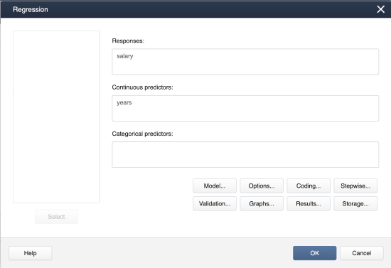
Figure \(\PageIndex{b1}\): Minitab Regressions pop-up window Click OK, and Minitab will output the following.
Regression Analysis: Salary versus years
Regression Equation: salary = 24.8 + 15.2 years
Coefficients
Term Coef SE Coef T-Value P-Value VIF Constant 24.80 7.53 3.29 0.046 years 15.20 2.27 6.69 0.007 1.00 Model Summary
S R-sq R-sq (adj) R-sq (pred) 7.18331 R-Sq = 93.7% 91.6% 85.94% Analysis of Variance
Source DF SS MS F-Value P-Value Regression 1 2310.4 2310.40 44.78 0.007 years 1 2310.4 2310.40 44.78 0.007 Residual Error 3 154.8 51.6 Total 4 2465.2 Females
Open Minitab dataset Female Salary Dataset. Follow the same procedure as was done for the Male dataset and Minitab will output the following:
Regression Analysis: Salary versus years
Regression Equation: salary = 3.00 + 15.00 years
Coefficients
Term Coef SE Coef T-Value P-Value VIF Constant 3.00 3.32 0.90 0.432 years 15.00 1.00 15.00 0.001 1.00 Model Summary
S R-sq R-sq (adj) R-sq (pred) 3.16228 98.68% 98.25% 95.92% Analysis of Variance
Source DF SS MS F-Value P-Value Regression 1 2250.0 2250.0 225.00 0.001 years 1 2250.0 2250.0 225.00 0.001 Residual Error 3 30.0 10.0 Total 4 2280.0 In both cases, the simple linear regressions are significant, so the slopes are not = 0.
Step 2: Are the slopes equal?
We can test for this using our statistical software. In Minitab, we must now use GLM (general linear model) and be sure to include the covariate in the model. We will also include a "treatment x covariate" interaction term and the significance of this term is what answers our question. If the slopes differ significantly among treatment levels, the interaction p-value will be < 0.05.
First, open the dataset in the Minitab project file Salary Dataset. Then, from the menu select Stat > ANOVA > General Linear Model > Fit General Linear Model
In the dialog box, select salary into Responses, gender into Factors, and years into Covariates.
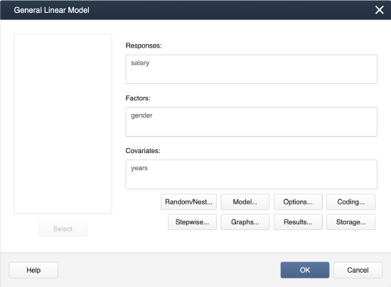 Figure \(\PageIndex{b2}\): Minitab GLM pop-up selections
To add the interaction term, first click Model…. Then, use the shift key to highlight gender and years, and click Add. Click OK, then OK again, and Minitab will display the following output.
Analysis of Variance
Source DF Adj SS Adj MS F-Value P-Value year 1 4560.20 4560.20 148.06 0.000 gender 1 216.02 216.02 7.01 0.038 years*gender 1 0.20 0.20 0.01 0.938 Error 6 184.80 30.80 Total 9 5999.60 It is clear the interaction term is not significant. This suggests the slopes are equal. In a plot of the regressions, we can also see that the lines are parallel.
Figure \(\PageIndex{b3}\): Parallel lines of best fit Step 3: Fit an Equal Slopes Model
We can now proceed to fit an Equal Slopes model by removing the interaction term. This can be easily accomplished by starting again with STAT > ANOVA > General Linear Model > Fit General Linear Model
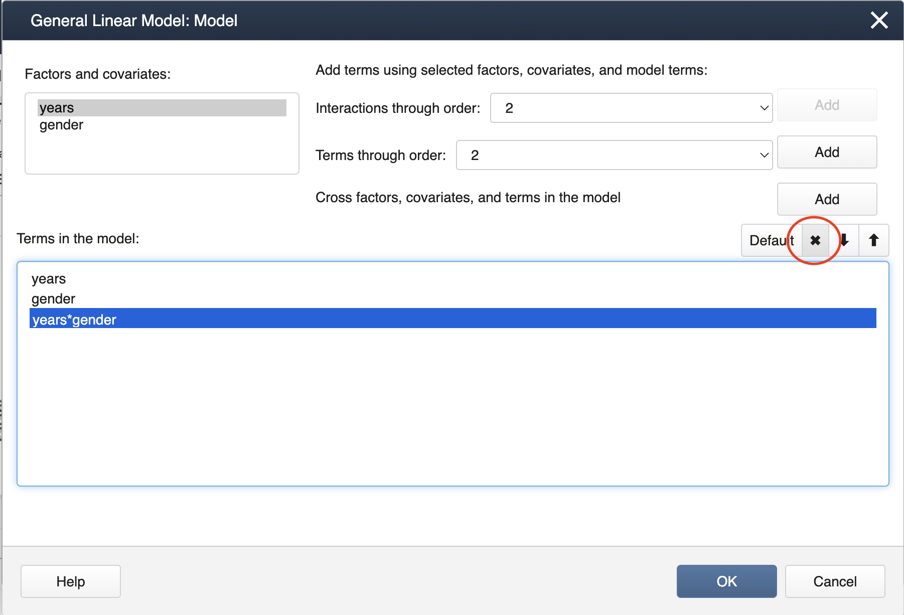
Figure \(\PageIndex{b4}\): Removing the years*genderterm from the modelClick OK, then OK again, and Minitab will display the following output.
Analysis of Variance
Source DF Adj SS Adj MS F-Value P-Value year 1 4560.20 4560.20 172.55 0.000 gender 1 1254.4 1254.40 47.46 0.000 Error 7 185.0 26.43 Total 9 5999.6 To generate the mean comparisons select STAT > ANOVA > General Linear Model > Comparisons... and fill in the dialog box as seen below.
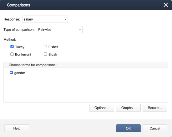
Figure \(\PageIndex{b5}\): Comparisons window selections Click OK and Minitab will produce the following output.
Comparison of salary
Tukey Pairwise Comparisons: gender
Grouping information Using the Tukey Method and 95% Confidencegender N Mean Grouping Male 5 70.4 A gender 5 48.0 B Means that do not share a letter are significantly different.
Steps for the ANCOVA for the Salary example in R:
- Run a simple linear model for each treatment group.
- Testing whether the slopes are equal.
- Plot the regression lines.
- Fit an equal slopes model.
- Steps in R
-
1. Run a simple linear model for each treatment group (males and females) by using the following commands:
Males
males_regression <- lm(salary~years,data=subset(equal_slopes_data,gender=="m"))
anova(males_regression)
#Analysis of Variance Table
#Response: salary
#          Df  Sum Sq  Mean Sq  F value    Pr(>F)
#years      1  2310.4   2310.4   44.775  0.006809 **
#Residuals  3   154.8     51.6
#---
#Signif. codes:  0 ‘***’ 0.001 ‘**’ 0.01 ‘*’ 0.05 ‘.’ 0.1 ‘ ’ 1
#summary(males_regression)$coefficients
#              Estimate  Std. Error    t value     Pr(>|t|)
#(Intercept)       24.8    7.533923   3.291778  0.046016514
#years             15.2    2.271563   6.691427  0.006808538
Females
females_regression <- lm(salary~years,data=subset(equal_slopes_data,gender=="f"))
anova(females_regression)
#Analysis of Variance Table
#Response: salary
#          Df  Sum Sq  Mean Sq  F value     Pr(>F)
#years      1    2250     2250      225  0.0006431 ***
#Residuals  3      30       10
#---
#Signif. codes:  0 ‘***’ 0.001 ‘**’ 0.01 ‘*’ 0.05 ‘.’ 0.1 ‘ ’ 1
#  summary(females_regression)$coefficients
#              Estimate  Std. Error   t value       Pr(>|t|)
#(Intercept)          3    3.316625  0.904534   0.4323889978
#years               15    1.000000 15.000000   0.0006431193
2. Test whether the slopes are equal by using the following commands:
ancova_model<-lm(salary ~ gender + years + gender:years,equal_slopes_data)
anova(ancova_model)
Analysis of Variance Table
Response: salary
             Df  Sum Sq  Mean Sq  F value     Pr(>F)
gender        1  1254.4   1254.4  40.7273  0.0006961 ***
years         1  4560.2   4560.2 148.0584  1.874e-05 ***
gender:years  1     0.2      0.2   0.0065  0.9383948
Residuals     6   184.8     30.8
---
Signif. codes:  0 ‘***’ 0.001 ‘**’ 0.01 ‘*’ 0.05 ‘.’ 0.1 ‘ ’ 1
With a p-value of 0.9383948 in the interaction term (
gender*years), we can conclude that the slopes are equal.3. Plot the regression line for males and females by using the following commands:
plot(years,salary, xlab="Years after graduation", ylab="Salary(Thousands)",pch=23, col=ifelse(gender=="m","red","blue"), lwd=2)
abline(males_regression)
abline(females_regression)
text(locator(1),"y=15.2x+24.8",col="red")
text(locator(1),"y=15x+3",col="blue")
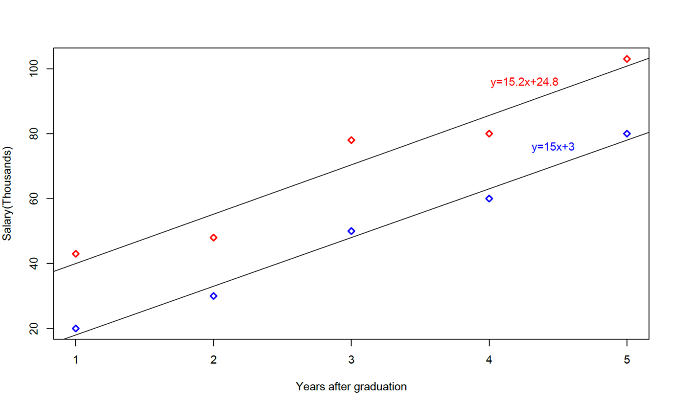
Figure \(\PageIndex{c1}\): Regression lines for male and female data 4. Fit an equal slopes model by using the following commands:
equal_slopes_model<-lm(salary ~ gender + years,equal_slopes_data)
anova(equal_slopes_model)
#Analysis of Variance Table
#Response: salary
#          Df  Sum Sq  Mean Sq  F value     Pr(>F)
#gender     1  1254.4   1254.4   47.464  0.0002335 ***
#years      1  4560.2   4560.2  172.548  3.458e-06 ***
#Residuals  7   185.0     26.4
#---
#Signif. codes:  0 ‘***’ 0.001 ‘**’ 0.01 ‘*’ 0.05 ‘.’ 0.1 ‘ ’ 1
We can see that gender is significant now. To estimate the two regression lines, we need the following output:
summary(equal_slopes_model)$coefficients
#Coefficients:
#            Estimate  Std. Error  t value  Pr(>|t|)
#(Intercept)    2.700       4.145    0.651  0.535560
#genderm       22.400       3.251    6.889  0.000234
#years         15.100       1.150   13.136  3.46e-06
detach(equal_slopes_data)
The estimate for the years (15.1) is the slope of the models. The intercept for females is 2.7 and the intercept for males is 2.7+22.4=25.1
Thus, the estimated regression equation for females is \(y=15.1x + 2.7\) and for males it's \(y=15.1x + 25.1\).