9.1: Role of the Covariate

To illustrate the role the covariate has in the ANCOVA, let’s look at a hypothetical situation wherein investigators are comparing the salaries of male vs. female college graduates. A random sample of 5 individuals for each gender is compiled, and a simple one-way ANOVA is performed:

Males	Females
78	80
43	50
103	30
48	20
80	60

\(H_{0}: \ \mu_{\text{males}} = \mu_{\text{females}}\)

SAS Example

Using SAS

SAS coding for the One-way ANOVA:

data ancova_example;
input gender $ salary;
datalines;
m 78
m 43
m 103
m 48
m 80
f 80
f 50
f 30
f 20
f 60
;
proc mixed data=ancova_example method=type3;
class gender;
model salary=gender;
run;

Here is the output we get:

Type 3 Tests of Fixed Effects
Effect	Num DF	Den DF	F Value	Pr > F
gender	1	8	2.11	F">0.1840

Minitab Example

Using Minitab

To perform a one-way ANOVA test in Minitab, you can first open the data (ANCOVA Example Minitab Data) and then select Stat > ANOVA > One Way…

In the pop-up window that appears, select salary as the Response and gender as the Factor.

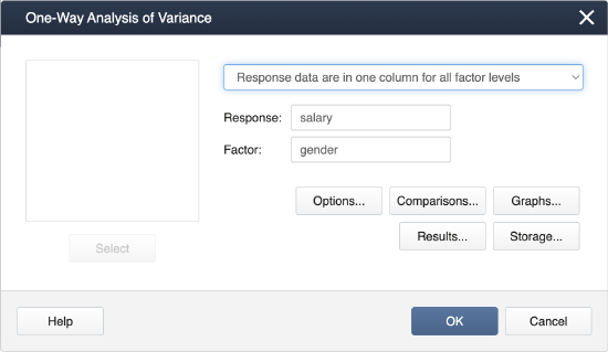
Figure \(\PageIndex{1}\): Minitab One-Way Analysis of Variance window

Click OK, and the output is as follows.

Analysis of Variance

Source	DF	SS	SS	F-Value	P-Value
gender	1	1254	1254	2.11	0.184
Error	8	4745	593
Total	9	6000

Model Summary

S	R-sq	R-sq(adj)	R-sq(pred)
24.3547	20.91%	11.02%	0.00%

R Example

Using R

Tasks:

• Load the ANCOVA example data.
• Obtain the ANOVA table.
• Plot the data.

1. Load the ANCOVA example data and obtain the ANOVA table by using the following commands:

setwd("~/path-to-folder/")
ancova_example_data <- read.table("ancova_example.txt",header=T)
attach(ancova_example_data)
ancova<-aov(salary ~ gender,ancova_example_data)
summary(ancova)
#            Df  Sum Sq  Mean Sq  F value  Pr(>F)
#gender       1    1254   1254.4    2.115   0.184
#Residuals    8    4745    593.1       

2. Plot for the data, salary by gender, by using the following commands:

library(ggplot2)
myplot<-ggplot(ancova_example_data, aes(x = gender, y = salary)) +  geom_point()
myplot + theme_bw() + theme(panel.border = element_blank(), panel.grid.major = element_blank(),
panel.grid.minor = element_blank(), axis.line = element_line(colour = "black"))

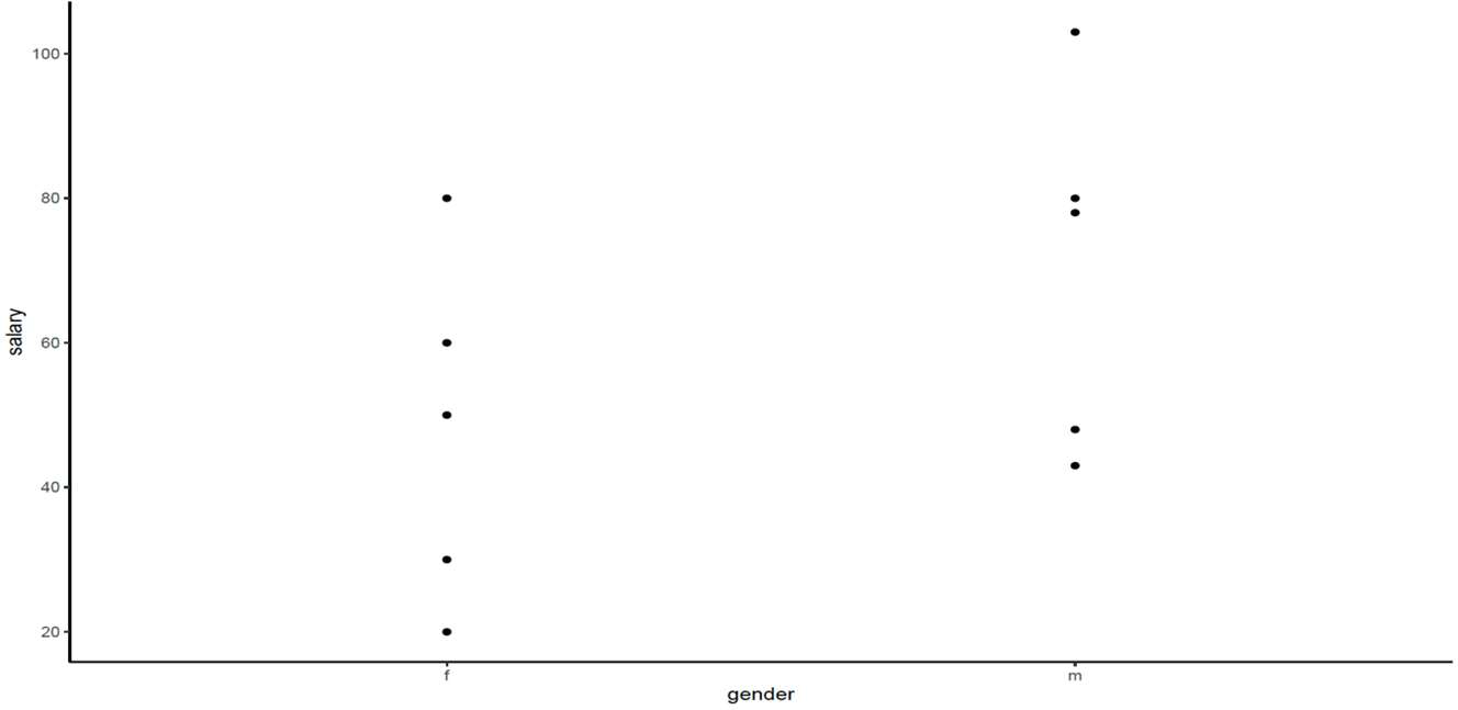
Figure \(\PageIndex{2}\): Gender and salary plot

3. Plot for the data, salary vs years, by using the following commands:

plot(years,salary, xlab="Years after graduation", ylab="Salary(Thousands)",pch=23,cex=2, col="cornflowerblue", bg="cornflowerblue", lwd=2)
abline(lm(salary~years,data=ancova_example_data))
detach(ancova_example_data)

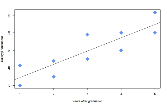
Figure \(\PageIndex{3}\): Plot of salary vs years

Because the \(p\)-value > \(\alpha\) (=0.05), they can't reject the \(H_{0}\).

A plot of the data shows the situation:

Figure \(\PageIndex{4}\): Plot of salary vs gender

However, it is reasonable to assume that the length of time since graduation from college is also likely to influence one's income. So more appropriately, the duration since graduation, a continuous variable, should be also included in the analysis, and the required data is shown below.

Females		Males
Salary	years	Salary	years
80	5	78	3
50	3	43	1
30	2	103	5
20	1	48	2
60	4	80	4

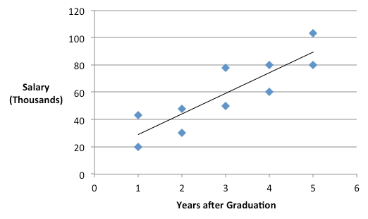
Figure \(\PageIndex{5}\): Plot of salary vs years since graduation

The plot above indicates an upward linear trend between salary and the number of years since graduation, which could be a marker for experience and/or postgraduate education. The fundamental idea of including a covariate is to take this trend into account and to "control" it effectively. In other words, including the covariate in the ANOVA will make the comparison between Males and Females after accounting for the covariate.