8.1: Split-Plot Design in RCBD

Recall the Randomized Complete Block Design (RCBD) we discussed in Chapter 7. In RCBD, general blocks are formed such that the experimental units are expected to be homogenous within a block and heterogeneous between blocks.

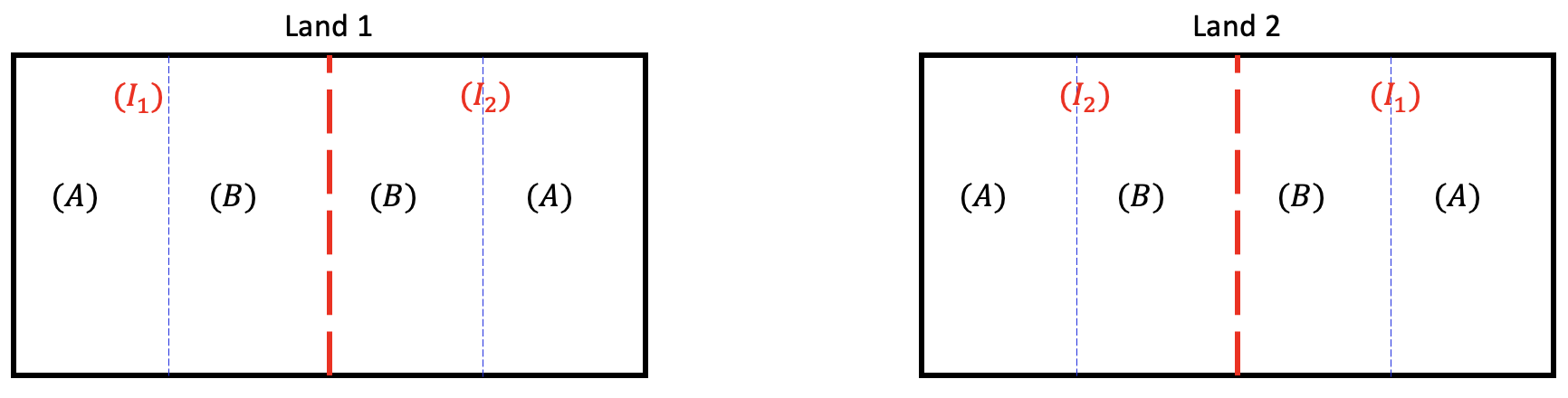
For example. suppose we are studying the effect of irrigation amount (\(I_{1}\) and \(I_{2}\)) and fertilizer type (\(A\) and \(B\)) on crop yield. We have 4 treatments in this experiment. Suppose we want to have at least 2 replicates and have two large lands that can be used for the experiment. In RCBD, we can split each land into 4 fields and can apply the 4 treatments randomly to each field. Here lands are blocks and fields are the experimental units.

Figure \(\PageIndex{1}\): Lands divided into 4 fields each, each field assigned one of the 4 random treatments.

In this example, we have assumed that managing levels of irrigation and fertilizer require the same effort. Now suppose varying the level of irrigation is difficult on a small scale and it makes more sense to apply irrigation levels to larger areas of land.

In such situations, we can divide each land into two large fields (whole plots) and apply irrigation amounts to each field randomly. And then divide each of these large fields into smaller fields (subplots) and apply fertilizer randomly within the whole plots.

Figure \(\PageIndex{2}\): Lands divided into 2 plots for irrigation, with each plot divided into 2 fields for fertilizer treatment.

In this strategy, each land contains two whole plots and irrigation amount is assigned to each whole plot randomly using RCBD (i.e. lands are treated as blocks and irrigation amount is assigned randomly within each block to the whole plots). Each whole plot contains two subplots and fertilizer type is assigned to each subplot using RCBD (i.e. whole plots are treated as blocks and fertilizer type is assigned randomly within each whole plot to the subplots).

When some factors are more difficult to vary than others at the levels of experimental units, it is more efficient to assign more difficult-to-change factors to larger units (whole plots) and then apply the easier-to-change factor to smaller units (subplots). This is known as the split-plot design.

As an example (adapted from Hicks, 1964), consider an experiment where an electrical component is subjected to 4 different temperatures for 3 different amounts of time. If the investigators desire 3 replications for each of the 12 temperature and time combinations (i.e. 12 treatments), a basic CRD or an RCBD (with a suitable blocking factor that would generate the replicates) will require as many as 36 attempts of testing.

Instead, the experimentation can be modified as follows to reduce effort and time. Regarding ovens as blocks, 3 ovens can be set to each of the 4 different temperature settings and then investigators can take out randomly selected components at the 3 different times of interest.

In this setting, temperatures are assigned randomly within each oven (i.e. an oven is treated as a block) and within each temperature, the baking times are assigned randomly to components. We have two RCBD sub-experiments: whole plot levels (temperatures) are assigned as RCBD within the oven and subplots levels (baking time) are assigned as RCBD within whole plot levels.

The data (Bake Time Data) were:

		Oven Temperature \((^{\circ} \mathrm{F})\)
Rep	Baking Time (min)	580	600	620	640
I	5	217	158	229	223
	10	233	138	186	227
	15	175	152	155	156
II	5	188	126	160	201
	10	201	130	170	181
	15	195	147	161	172
III	5	162	122	167	182
	10	170	185	181	201
	15	213	180	182	199

It is important to notice that in a split-plot design, randomization is a two-stage process. Levels of one factor (say, factor A) are randomized over the whole plots within each block, and the levels of the other factor (say, factor B) are randomized over the subplots within each whole plot. This restriction in randomization results in two different error terms: one appropriate for comparisons at the whole plot level and one appropriate for comparisons at the subplot level.

The appropriate error for whole plot level in split-plot RCBD is \(\text{whole plot factor} \times \text{block interaction}\). In other words, the analysis at the whole plot level is essentially of a one-way ANOVA with blocking (i.e. one observation per block-treatment combination). From the perspective of the whole plot, the subplots are simply subsamples and it is reasonable to average them when testing the whole plot effects (i.e. factor A effects).

The subplot factor (i.e. factor B) is always compared within the whole plot factor.

Source	DF
Blocks	\(r-1\)
Factor \(A\)	\(a-1\)
Whole plot Error	\((r-1)(a-1)\)
Factor B	\(b-1\)
\(A \times B\)	\((a-1)(b-1)\)
Subplot Error	\(a(r-1)(b-1)\)
Total	\(rab-1\)

The statistical model associated with the split-plot design with whole plots arranged as RCBD is \[Y_{ijk} = \mu + \alpha_{i} + \gamma_{k} + (\alpha \gamma)_{ik} + \beta_{j} + (\alpha \beta)_{ij} + \epsilon_{ijk}\] where \(\gamma_{k}\) for \(k=1,\ldots,r\) are block effects, \(\alpha_{i}\) for \(i=1,\ldots,a\) are factor A effects, and \(\beta_{j}\) for \(j=1,\ldots,b\) are factor B effects.

Using Technology

SAS Example

Steps in SAS

In SAS, we could specify the model with the following statements:

proc mixed data=BakeTimeData method=type3;
class oven temp time;
model resp=temp time temp*time;
random oven oven*temp;
run;

This will generate the ANOVA table as shown below.

Type 3 Analysis of Variance
Source	DF	Sum of Squares	Mean Square	Expected Mean Square	Error Term	Error DF	F Value	Pr > F
temp	3	12494	4164.768519	Var(Residual) + 3 Var(oven*temp) + Q(temp,temp*time)	MS(oven*temp)	6	14.09	0.0040
time	2	566.222222	283.111111	Var(Residual) + Q(time,temp*time)	MS(Residual)	16	0.46	0.6418
temp*time	6	2600.444444	433.407407	Var(Residual) + Q(temp*time)	MS(Residual)	16	0.70	0.6551
oven	2	1962.722222	981.361111	Var(Residual) + 3 Var(oven*temp) + 12 Var(oven)	MS(oven*temp)	6	3.32	0.1070
oven*temp	6	1773.944444	295.657407	Var(Residual) + 3 Var(oven*temp)	MS(Residual)	16	0.48	0.8162
Residual	16	9933.333333	620.833333	Var(Residual)	.	.	.	.

The ANOVA table can be rearranged to the following to make it easier to understand the whole plot and subplot analyses.

Source	DF	Expected Mean Square
(Whole Plots)
oven	2	Var(Residual) + 3 Var(block*temp) + 12 Var(oven)
temp	3	Var(Residual) + 3 Var(oven*temp) + Q(temp, temp*time)
oven*temp	6	Var(Residual) + 3 Var(oven*temp)
(Subplots)
time	2	Var(Residual) + Q(time, temp*time)
temp*time	6	Var(Residual) + Q(temp*time)
Residual	16	Var(Residual)

Notice that the correct error term for the \(F\)-test of the treatment applied to whole plots is the \(\text{block} \times \text{whole plot factor}\) (assuming blocks are a random effect).

Note!

One might wonder about the terms \(\text{block} \times \text{subplot factor}\) and \(\text{block} \times \text{whole plot factor} \times \text{subplot factor}\). With these terms in the model, we will not be able to retrieve the residual (the error DF will be zero). If repeat observations are made within the split-plots, then a separate error term can be estimated. However, it is important to keep in mind that tests of replication effects are not of interest, but are being isolated in the ANOVA to reduce the error variance. As a result, the model that is usually run in this design drops out the \(\text{block} \times \text{subplot factor}\) and \(\text{block} \times \text{whole plot factor} \times \text{subplot factor}\) terms, and combine these interactions with the true error variance to obtain a working error term.

R Example

Steps in R

Load the bake time data and obtain the ANOVA table by using the following commands:

setwd("~/path-to-folder/")
baketime_data <- read.table("baketime_data.txt",header=T)
attach(baketime_data)
baketime_anova<-aov(resp ~ factor(temp) + factor(time) + factor(temp):factor(time) + Error(factor(oven)+factor(oven):factor(temp)),baketime_data)
summary(baketime_anova)
#Error: factor(oven)
#          Df Sum Sq Mean Sq F value Pr(>F)
#Residuals  2   1963   981.4               
#Error: factor(oven):factor(temp)
#             Df Sum Sq Mean Sq F value Pr(>F)   
#factor(temp)  3  12494    4165   14.09  0.004 **
#Residuals     6   1774     296                  
#---
#Signif. codes:  0 ‘***’ 0.001 ‘**’ 0.01 ‘*’ 0.05 ‘.’ 0.1 ‘ ’ 1
#Error: Within
#                          #Df Sum Sq Mean Sq F value Pr(>F)
#factor(time)               2    566   283.1   0.456  0.642
#factor(temp):factor(time)  6   2600   433.4   0.698  0.655
#Residuals                 16   9933   620.8               
detach(baketime_data)