4.4: Dummy Variable Regression

Model 3 - Dummy Variable Regression

\[Y_{ij} = \mu + \mu_{i} + \epsilon_{ij}, \text{ fitted as } Y_{ij} = \beta_{0} + \beta_{Level \ 1} + \beta_{Level \ 2} + \ldots + \beta_{Level \ T-1} + \epsilon_{ij}\]

where \(\beta_{Level \ 1}, \beta_{Level \ 2}, \ldots, \beta_{Level \ T-1}\) are regression coefficients for \(T-1\) indicator-coded regression "dummy" variables that are correspond to the \(T-1\) categorical factor levels. The \(T^{th}\) factor level mean is given by the regression intercept \(\beta_{0}\).

The General Linear Model (GLM) applied to data with categorical predictors can be viewed from a regression modeling perspective as an ordinary multiple linear regression (MLR) with "dummy" coding, also known as indicator coding, for the categorical treatment levels. Typically, software performing the MLR will automatically include an intercept, which corresponds to the first column of the design matrix and is a column of \(1\)'s. This automatic inclusion of the intercept can lead to complications when interpreting the regression coefficients.

The SAS Mixed procedure, and also the GLM procedure which we may encounter later, use the "Dummy Variable Regression" model. For the \(Y\) data used in sections 4.2 and 4.3, the design matrix for this model can be entered into IML as:

/* Dummy Variable Regression Model */
x = {
1    1    0,
1    1    0,
1    0    1,
1    0    1,
1    0    0,
1    0    0};

Notice that in the above design matrix, there are only two indicator columns even though there are three treatment levels in the study. It is because, similar to the matrix below, if we were to have a design matrix with another indicator column representing the third treatment level, the resulting 4 columns would form a set of linearly dependent columns, a mathematical condition that will hinder the computation process any further as explained below. \[\begin{bmatrix} 1 & 1 & 0 & 0 \\ 1 & 1 & 0 & 0 \\ 1 & 0 & 1 & 0 \\ 1 & 0 & 1 & 0 \\ 1 & 0 & 0 & 1 \\ 1 & 0 & 0 & 1 \end{bmatrix}\]

The above matrix containing all 4 columns has the property that the sum of columns 2-4 will equal the first column representing the intercept. As a result, a mathematical condition called singularity is created and the matrix computations will not run. So one of the treatment levels is omitted from the coding in the design matrix above for IML and the eliminated level is called the ‘reference’ level. In SAS, typically, the treatment level with the highest label is defined as the reference level and so, in this study, it is treatment level 3.

Note that the parameter vector for the dummy variable regression model is \[\boldsymbol{\beta} = \begin{bmatrix} \mu_{1} \\ \mu_{2} \\ \mu_{3} \end{bmatrix}\].

Running IML, with the design matrix for the dummy variable regression model, we get the following output;

Regression Coefficients
Beta_0	5.5
Beta_1	-4
Beta_2	-2

The coefficient \(\beta_{0}\) is the mean for treatment level 3. The mean for treatment level 1 is then calculated from \(\hat{\beta}_{0} + \hat{\beta}_{1} = 1.5\). Likewise, the mean for treatment level 2 is calculated as \(\hat{\beta}_{0} + \hat{\beta}_{2} = 3.5\).

Notice that the \(F\) statistic calculated from this model is the same as that produced from the Cell Means model.

ANOVA
Treatment	df	SS	MS	F
	2	16	8	16
Error	3	1.5	0.5
Total	5	17.5

Using Technology

Minitab Example

We can confirm our ANOVA table now by running the analysis in software such as Minitab.

Steps in Minitab

First input the data:

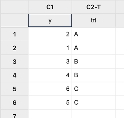
Figure \(\PageIndex{a1}\): Inputting data.

In Minitab, different coding options allow the choice of the design matrix which can be done as follows:

Stat > ANOVA > General Linear Model > Fit General Linear Model and place the variables in the appropriate boxes:

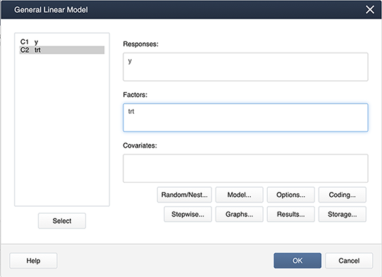
Figure \(\PageIndex{a2}\): Placing variables in the General Linear Model pop-up window.

Then select Coding… and choose the (1,0) coding as shown below:

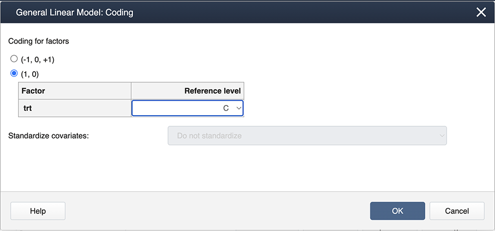
Figure \(\PageIndex{a3}\): Selecting options in the General Linear Model: Coding window.

Select OK to exit the nested windows. This produces the regular ANOVA output:

Analysis of Variance

Source	DF	Adj SS	Adj MS	F-Value	P-Value
trt	2	16.000	8.0000	16.00	0.025
Error	3	1.500	0.5000
Total	5	17.500

And also the Regression Equation:

Regression Equation

y = 5.500 - 4.000 trt_level1 - 2.000 trt_level2 + 0.0 trt_level3

SAS Example

Steps in SAS

In SAS, the default coding is indicator coding, so when you specify the option

model y=trt / solution;

Copy code

you get the regression coefficients:

Solution for Fixed Effects
Effect	trt	Estimate	Standard Error	DF	t Value	Pr > |t|
Intercept		5.5000	0.5000	3	11.00	0.0016
trt	level1	-4.0000	0.7071	3	-5.66	0.0109
trt	level2	-2.0000	0.7071	3	-2.83	0.0663
trt	level3	0

And the same ANOVA table:

Type 3 Analysis of Variance
Source	DF	Sum of Squares	Mean Square	Expected Mean Square	Error Term	Error DF	F Value	Pr > F
trt	2	16.000000	8.000000	Var(Residual)+Q(trt)	MS(Residual)	3	16.00	0.0251
Residual	3	1.500000	0.500000	Var(Residual)

The Intermediate calculations for this model are:

xprimex 6 2 2 2 2 0 2 0 2	check 1 -2.22E-16 0 3.331E-16 1 0 0 0 1	xprimey 21 3 7
SumY2 89.5	CF 73.5	xprimexinv 0.5 -0.5 -0.5 -0.5 1 0.5 -0.5 0.5 1

R Example

Steps in R

1. Define response variable and design matrix

y<-matrix(c(2,1,3,4,6,5), ncol=1)
x = matrix(c(1,1,0,1,1,0,1,0,1,1,0,1,1,0,0,1,0,0),ncol=3,nrow=6,byrow=TRUE)

2. Regression coefficients

beta<-solve(t(x)%*%x)%*%(t(x)%*%y)
#  beta
#      [,1]
# [1,]  5.5
# [2,] -4.0
# [3,] -2.0

3. Calculate the entries of the ANOVA Table

n<-nrow(y)
p<-ncol(x)
J<-matrix(1,n,n)
ss_tot = (t(y)%*%y) - (1/n)*(t(y)%*%J)%*%y #17.5
ss_trt = t(beta)%*%(t(x)%*%y) - (1/n)*(t(y)%*%J)%*%y #16
ss_error = ss_tot - ss_trt #1.5
total_df=n-1 #5
trt_df=p-1 #2
error_df=n-p #3
MS_trt = ss_trt/(p-1) #8
MS_error = ss_error / error_df #0.5
F=MS_trt/MS_error #16

4. Creating the ANOVA table

ANOVA <- data.frame(
c ("","Treatment","Error", "Total"),
c("DF", trt_df,error_df,total_df),
c("SS", ss_trt, ss_error, ss_tot),
c("MS", MS_trt, MS_error, ""),
c("F",F,"",""),
stringsAsFactors = FALSE)
names(ANOVA) <- c(" ", "  ", " ","","")

5. Print the ANOVA table

print(ANOVA)    
# 1           DF   SS  MS  F
# 2 Treatment  2   16   8 16
# 3     Error  3  1.5 0.5   
# 4     Total  5 17.5   

6. Intermediates in the matrix computations

xprimex<-t(x)%*%x
#  xprimex
#      [,1] [,2] [,3]
# [1,]    6    2    2
# [2,]    2    2    0
# [3,]    2    0    2
xprimey<-t(x)%*%y
#   xprimey
#      [,1]
# [1,]   21
# [2,]    3
# [3,]    7
xprimexinv<-solve(t(x)%*%x)
#  xprimexinv
#      [,1] [,2] [,3]
# [1,]  0.5 -0.5 -0.5
# [2,] -0.5  1.0  0.5
# [3,] -0.5  0.5  1.0
check<-xprimexinv%*%xprimex
#  check
#               [,1]          [,2] [,3]
# [1,]  1.000000e+00  0.000000e+00    0
# [2,] -1.110223e-16  1.000000e+00    0
# [3,]  0.000000e+00 -1.110223e-16    1
SumY2<-t(beta)%*%(t(x)%*%y) # 89.5
CF<-(1/n)*(t(y)%*%J)%*%y # 73.5

7. Regression Equation and ANOVA table

trt_level1<-x[,2]
trt_level2<-x[,3]
model<-lm(y~trt_level1+trt_level2)

8. With the command summary(model) we can get the following output:

Call:
lm(formula = y ~ trt_level1 + trt_level2)
Residuals:
1    2    3    4    5    6
0.5 -0.5 -0.5  0.5  0.5 -0.5
Coefficients:
Estimate Std. Error t value Pr(>|t|)   
(Intercept)   5.5000     0.5000  11.000  0.00161 **
trt_level1   -4.0000     0.7071  -5.657  0.01094 *
trt_level2   -2.0000     0.7071  -2.828  0.06628 .
---
Signif. codes:  0 ‘***’ 0.001 ‘**’ 0.01 ‘*’ 0.05 ‘.’ 0.1 ‘ ’ 1
Residual standard error: 0.7071 on 3 degrees of freedom
Multiple R-squared:  0.9143,    Adjusted R-squared:  0.8571
F-statistic:    16 on 2 and 3 DF,  p-value: 0.02509

From the output, we can see the estimates for the coefficients are b0=5.5, b1=-4, b2=-2 and the F-statistic is 16 with a p-value of 0.02509.

By using the estimates we can write the regression equation:

y=5.5-4 trt_level1-2 trt_level2+0 trt_level3

9. With the command anova(model) we can get the following output

Analysis of Variance Table
Response: y           
Df Sum Sq Mean Sq F value  Pr(>F)  
trt_level1  1   12.0    12.0      24 0.01628 *
trt_level2  1    4.0     4.0       8 0.06628 .
Residuals   3    1.5     0.5                   ---
Signif. codes:  0 ‘***’ 0.001 ‘**’ 0.01 ‘*’ 0.05 ‘.’ 0.1 ‘ ’ 1

Note: R is giving the sequential sum of squares in the ANOVA table.