2.2: Computing Quantities for the ANOVA Table

When working with ANOVA, we start with the total variability in the response variable and divide or "partition" it into different parts: the between sample variability (i.e. variability due to our treatment) and the within sample variability (i.e. residual variability). The variability that is due to our treatment we of course hope is significantly large and variability in the response that is leftover can be thought of as the nuisance, "error", or "residual" variability.

To help you imagine this a bit more, think about the data storage capacity of a computer. If you have 8GB of storage total, you can ask your computer to show the types of files that are occupying the storage. The ANOVA model is (in a very elementary fashion) going to compare the variability due to the treatment to the variability left over.

From elementary statistics, when we think of computing a variance of a random variable (say \(X\)), we use the expression: \[\text{variance} = \frac{\sum \left(X_{i} - \bar{X}\right)^{2}}{N-1} = \frac{SS}{df}\]

The numerator of this expression is referred to as the Sum of Squares, or Sum of Squared deviations from the mean, or simply SS. (If you don't recognize this, then we suggest you sharpen your introductory statistics skills!) The denominator is the degrees of freedom, \((N-1)\), or \(df\).

ANOVA Table Rules

1. Total SS = sum of the SS of all Sources (i.e., Total SS = Treatment SS + Error SS)
2. Total df = sum of df of all Sources
3. MS = SS/df
4. \(F_{\text{calculated}} = \dfrac{\text{Treatment MS}}{\text{Error MS}}\) with numerator df = number of treatments - 1 and denominator df = error df

The ANOVA table is set up to generate quantities analogous to the simple variance calculation above. In our greenhouse experiment example:

1. We start by considering the TOTAL variability in the response variable. This is done by calculating the \(SS_{\text{Total}}\) \[\begin{array}{l} \text{Total SS} &= \sum_{i} \sum_{j} \left(Y_{ij} - \bar{Y}_{..}\right)^{2} \\ &= \mathbf{312.47} \end{array}\] The degrees of freedom for the Total SS is \(N - 1 = 24 - 1 = 23\), where \(N\) is the total sample size.
2. Our next step determines how much of the variability in \(Y\) is accounted for by our treatment. We now calculate \(SS_{\text{Treatment}}\) or \(SS_{\text{Trt}}\): \[\text{Treatment SS} = \sum_{i} n_{i} \left(\bar{Y}_{i.} - \bar{Y}_{..}\right)^{2}\]

   Note!

   The sum of squares for the treatment is the deviation of the group mean from the grand mean. So in some sense, we are "aggregating" all of the responses from that group and representing the "group effect" as the group mean.

   and for our example: \[\begin{array}{c} \text{Treatment SS} = 6 \times (21.0-26.1667)^{2} + 6 \times (28.6-26.1667)^{2} + \\ \ldots + 6 \times (25.8667-26.1667)^{2} + 6 \times (29.2-26.1667)^{2} = 251.44 \end{array}\] Note that in this case we have equal numbers of observations (6) per treatment level, and it is, therefore, a balanced ANOVA.

3. Finally, we need to determine how much variability is "left over". This is the Error or Residual sums of squares by subtraction: \[\begin{array}{l} \text{Error SS} &= \sum_{i} \sum_{j} \left(Y_{ij} - \bar{Y}_{i.}\right)^{2} = \text{Total SS} - \text{Treatment SS} \\ &= 312.47 - 251.44 = \mathbf{61.033} \end{array}\] Note here that the "leftover" is really the deviation of any score from its group mean.

We can now fill in the following columns of the table:

ANOVA

Source	df	SS	MS	F
Treatment	T - 1 = 3	251.44
Error	23-3=20	61.033
Total	N - 1 =23	312.47

We have \(T\) treatment levels and so we use \(T-1\) for the \(df\) for the treatment. In our example, there are 4 treatment levels (the control and the 3 fertilizers) so \(T=4\) and \(T-1 = 4-1 = 3\). Finally, we obtain the error \(df\) by subtraction as we did with the SS.

The Mean Squares (MS) can now be calculated as: \[MS_{Trt} = \frac{SS_{Trt}}{df_{Trt}} = \frac{251.44}{3} = 83.813\] and \[MS_{Error} = \frac{SS_{Error}}{df_{Error}} = \frac{61.033}{20} = 3.052\]

NOTE: \(MS_{\text{Error}}\) will sometimes be referred as \(MSE\) and we don’t need to calculate the \(MS_{\text{Total}}\).

ANOVA

Source	df	SS	MS	F
Treatment	3	251.44	83.813
Error	20	61.033	3.052
Total	23	312.47

Finally, we can compute the \(F\) statistic for our ANOVA. Conceptually we are comparing the ratio of the variability due to our treatment (remember we expect this to be relatively large) to the variability leftover, or due to error (and of course, since this is an error we want this to be small). Following this logic, we expect our \(F\) to be a large number. If we go back and think about the computer storage space we can picture most of the storage space taken up by our treatment, and less of it taken up by error. In our example, the \(F\) is calculated as: \[F = \frac{MS_{Trt}}{MS_{Error}} = \frac{83.813}{3.052} = 27.46\]

Source	df	SS	MS	F
Treatment	3	251.44	83.813	27.46
Error	20	61.033	3.052
Total	23	312.47

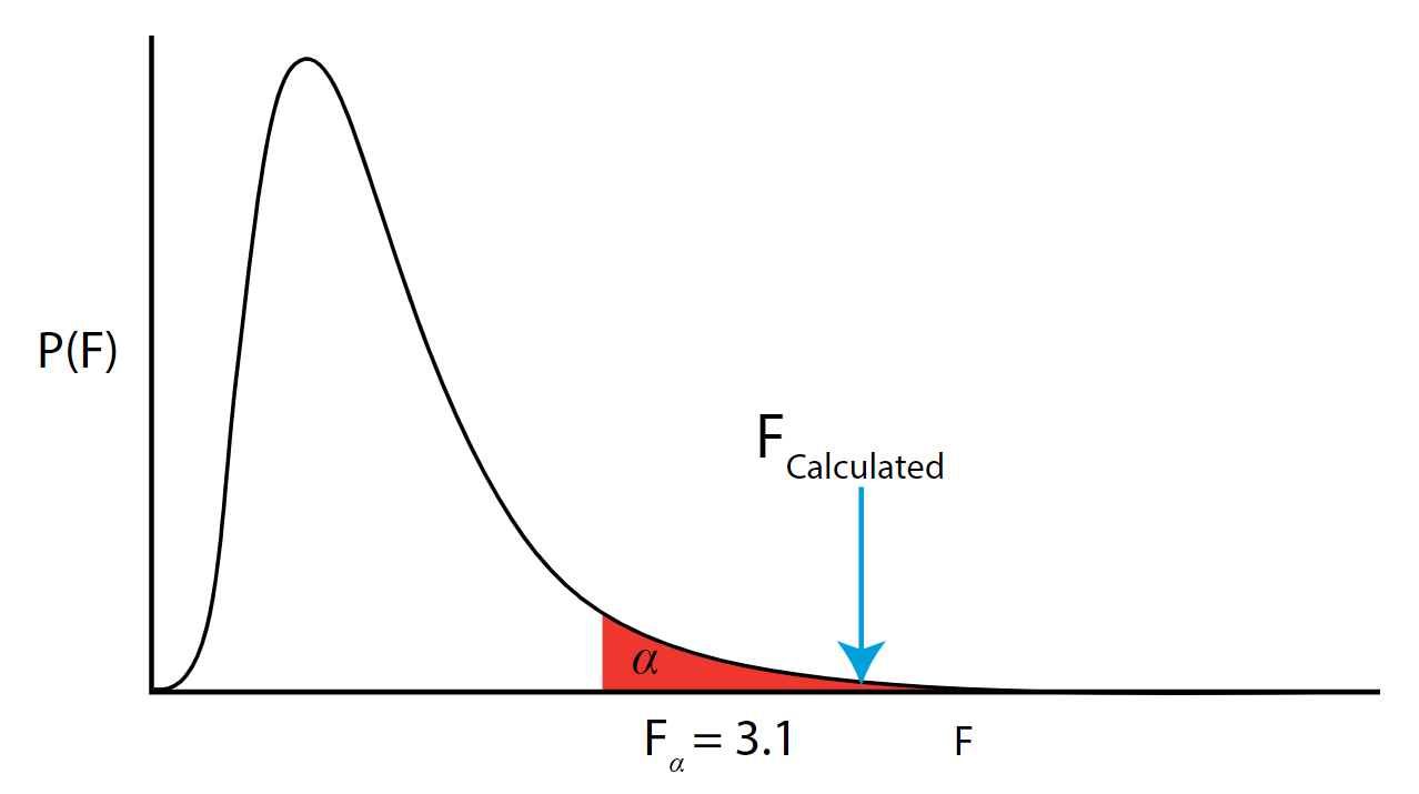
So how do we know if the \(F\) is large enough to conclude we have a significant amount of variability due to our treatment? We look up the critical value of \(F\) and compare it to the value we calculated. Specifically, the critical \(F\) is \(F_{\alpha} = F_{(0.05,3,20)} = 3.10\). The critical value can be found using tables or technology.

Finding a Critical Value of \(F\)

Using a Table:

Appendix Table B4

Using SAS:

data Fvalue;
    q=finv(0.95, 3, 20);
    put q=;
run;

proc print data=work.Fvalue;
    run;

The Print Procedure

Data Set WORK.FVALUE

Obs	q
1	3.09839

Most F tables actually index this value as \(1 - \alpha = .95\)

Figure \(\PageIndex{1}\): The \(F\) distribution.

The \(F_{calculated} > F_{\alpha}\) so we reject \(H_0\) and accept the alternative \(H_{A}\). The \(p\)-value (which we don't typically calculate by hand) is the area under the curve to the right of the \(F_{calculated}\) and is the way the process is reported in statistical software. Note that in the unlikely event that the \(F_{calculated}\) is exactly equal to the \(F_{\alpha}\) then the \(p \text{-value} = \alpha\). As the calculated \(F\) statistic increases beyond the \(F_{\alpha}\) and we go further into the rejection region, the area under the curve (hence the \(p\)-value) gets smaller and smaller. This leads us to the decisions rule: If the \(p\)-value is \(< \alpha\) then we reject \(H_{0}\).