
2.1: Building the ANOVA Table - Notation
- Page ID
- 33181

The idea of ANOVA is to compare different sources of variability: between sample variability and within sample variability.
As a point of review, the alternative hypothesis is what we think is going on (or what we need to conclude). Typically we are looking to find differences among at least one pair of our treatment means. Because of this, the null hypothesis (the opposite of the alternative) states that there are no differences among the group means (or that they are all equal).
To test the Null hypothesis (which is traditionally written as \(H_{0}: \ \mu_{1} = \mu_{2} = \ldots = \mu_{T}\), we need to compute the test \((F)\) statistic that compares the between sample variability to within sample variability.
To see how we compute this statistic it is helpful to look at the ANOVA table. The table below is an ANOVA table (here presented blank, with no entries yet):
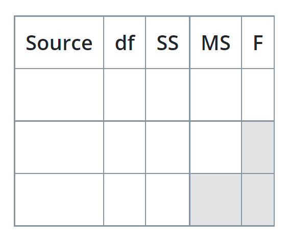.png?revision=1&size=bestfit&width=449&height=372)
To define the elements of the table and fill in these quantities, let’s return to our example data (Lesson 1 Data) for the hypothetical greenhouse experiment:
| Control | F1 | F2 | F3 |
|---|---|---|---|
| 21 | 32 | 22.5 | 28 |
| 19.5 | 30.5 | 26 | 27.5 |
| 22.5 | 25 | 28 | 31 |
| 21.5 | 27.5 | 27 | 29.5 |
| 20.5 | 28 | 26.5 | 30 |
| 21 | 28.6 | 25.2 | 29.2 |
Notation
Each observation in the dataset can be referenced by two indicator subscripts, \(i\) and \(j\), as \(Y_{ij}\).
For those of you not familiar with this notation, we use \(Y\) to indicate that it is a response variable. The subscript \(i\) refers to the \(i^{th}\) level of the treatment; our example has 4 treatments, so \(i\) will take on the values \(1, 2, 3,\) and \(4\).) The subscript \(j\) refers to the \(j^{th}\) observation (again, our example has 6 observations for each treatment so \(j\) takes the values \(1,2,3,4,5,\) and \(6\)). It is important to note that the \(j^{th}\) observation is occurring within the \(i^{th}\) treatment level.
| subscripts | \(i=1\) | \(i=2\) | \(i=3\) | \(i=4\) |
|---|---|---|---|---|
| Control | F1 | F2 | F3 | |
| \(j=1\) | 21 | 32 | 22.5 | 28 |
| \(j=2\) | 19.5 | 30.5 | 26 | 27.5 |
| \(j=3\) | 22.5 | 25 | 28 | 31 |
| \(j=4\) | 21.5 | 27.5 | 27 | 29.5 |
| \(j=5\) | 20.5 | 28 | 26.5 | 30 |
| \(j=6\) | 21 | 28.6 | 25.2 | 29.2 |
| For example, \(Y_{4,2}=27.5\). | ||||
We now can define the various means explicitly using these subscripts. The overall or Grand Mean is given by \[\text{Grand Mean} = \bar{Y}_{..}\]where the dots indicate that the quantity has been averaged over that subscript. For the Grand Mean, we have averaged over all \(j\) observations in all \(i\) treatment levels. The treatment means are given by \[\text{Treatment Mean} = \bar{Y}_{i}\] indicating that we have averaged over the \(j\) observations in each of the \(i\) treatment levels.
We can find these in the output from the summary procedure that can be generated in SAS and the coding details are discussed in Chapter 3:
| Fert | _Type_ | _FREQ_ | mean |
|---|---|---|---|
| 0 | 24 | 26.1667 | |
| Control | 1 | 6 | 21.0000 |
| F1 | 1 | 6 | 28.6000 |
| F2 | 1 | 6 | 25.8667 |
| F3 | 1 | 6 | 29.2000 |
In the output we see the column heading _TYPE_. The summary procedure in SAS calculates all possible means when specified, and so the _TYPE_ indicates what mean is being computed. _TYPE_ = 0 is the Grand Mean, and we can see this from the number of observations (given by _FREQ_) of 24. Each of the treatment level means is listed as _TYPE_ = 1 and we confirm that 6 replications were made for each treatment level (remember that j took on values 1 through 6).
Note that SAS automatically has ordered the treatment levels alphabetically.
The grand mean and treatment means are all we need in this example to compute the quantities for the ANOVA table.