1.2: The 7-Step Process of Statistical Hypothesis Testing

We will cover the seven steps one by one.

Step 1: State the Null Hypothesis

The null hypothesis can be thought of as the opposite of the "guess" the researchers made: in this example, the biologist thinks the plant height will be different for the fertilizers. So the null would be that there will be no difference among the groups of plants. Specifically, in more statistical language the null for an ANOVA is that the means are the same. We state the null hypothesis as: \[H_{0}: \ \mu_{1} = \mu_{2} = \ldots = \mu_{T}\] for \(T\) levels of an experimental treatment.

Note

Why do we do this? Why not simply test the working hypothesis directly? The answer lies in the Popperian Principle of Falsification. Karl Popper (a philosopher) discovered that we can't conclusively confirm a hypothesis, but we can conclusively negate one. So we set up a null hypothesis which is effectively the opposite of the working hypothesis. The hope is that based on the strength of the data, we will be able to negate or reject the null hypothesis and accept an alternative hypothesis. In other words, we usually see the working hypothesis in \(H_{A}\).

Step 2: State the Alternative Hypothesis

\[H_{A}: \ \text{treatment level means not all equal}\]

The reason we state the alternative hypothesis this way is that if the null is rejected, there are many possibilities.

For example, \(\mu_{1} \neq \mu_{2} = \ldots = \mu_{T}\) is one possibility, as is \(\mu_{1} = \mu_{2} \neq \mu_{3} = \ldots = \mu_{T}\). Many people make the mistake of stating the alternative hypothesis as \(mu_{1} \neq mu_{2} \neq \ldots \neq \mu_{T}\), which says that every mean differs from every other mean. This is a possibility, but only one of many possibilities. To cover all alternative outcomes, we resort to a verbal statement of "not all equal" and then follow up with mean comparisons to find out where differences among means exist. In our example, this means that fertilizer 1 may result in plants that are really tall, but fertilizers 2, 3, and the plants with no fertilizers don't differ from one another. A simpler way of thinking about this is that at least one mean is different from all others.

Step 3: Set \(\alpha\)

If we look at what can happen in a hypothesis test, we can construct the following contingency table:

Decision	In Reality
	\(H_{0}\) is TRUE	\(H_{0}\) is FALSE
Accept \(H_{0}\)	correct	Type II Error \(\beta\) = probability of Type II Error
Reject \(H_{0}\)	Type I Error \(\alpha\) = probability of Type I Error	correct

You should be familiar with type I and type II errors from your introductory course. It is important to note that we want to set \(\alpha\) before the experiment (a priori) because the Type I error is the more grievous error to make. The typical value of \(\alpha\) is 0.05, establishing a 95% confidence level. For this course, we will assume \(\alpha\)=0.05, unless stated otherwise.

Step 4: Collect Data

Remember the importance of recognizing whether data is collected through an experimental design or observational study.

Step 5: Calculate a test statistic

For categorical treatment level means, we use an \(F\) statistic, named after R.A. Fisher. We will explore the mechanics of computing the \(F\) statistic beginning in Chapter 2. The \(F\) value we get from the data is labeled \(F_{\text{calculated}}\).

Step 6: Construct Acceptance / Rejection regions

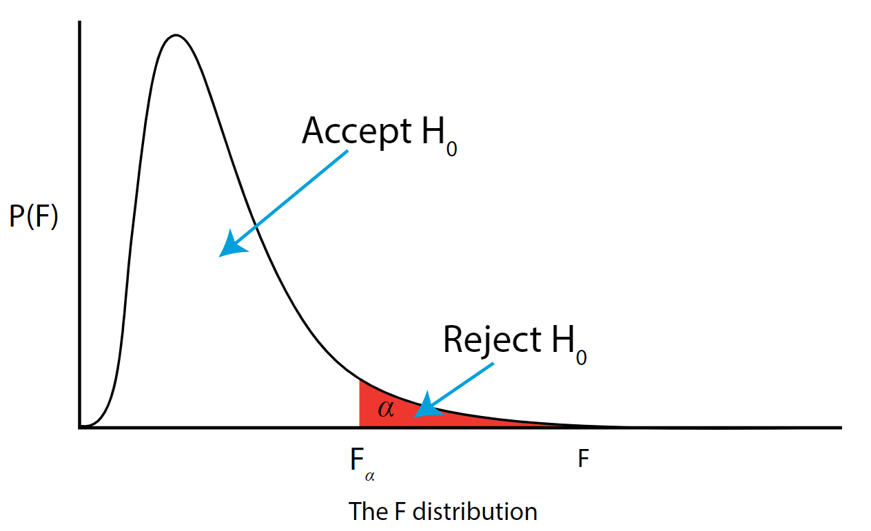
As with all other test statistics, a threshold (critical) value of \(F\) is established. This \(F\) value can be obtained from statistical tables or software and is referred to as \(F_{\text{critical}}\) or \(F_{\alpha}\). As a reminder, this critical value is the minimum value for the test statistic (in this case the F test) for us to be able to reject the null.

The \(F\) distribution, \(F_{\alpha}\), and the location of acceptance and rejection regions are shown in the graph below:

Figure \(\PageIndex{1}\): The F distribution, with \(F_{\alpha}\) and acceptance and rejection regions.

Step 7: Based on steps 5 and 6, draw a conclusion about H0

If the \(F_{\text{\calculated}}\) from the data is larger than the \(F_{\alpha}\), then you are in the rejection region and you can reject the null hypothesis with \((1 - \alpha)\) level of confidence.

Note that modern statistical software condenses steps 6 and 7 by providing a \(p\)-value. The \(p\)-value here is the probability of getting an \(F_{\text{calculated}}\) even greater than what you observe assuming the null hypothesis is true. If by chance, the \(F_{\text{calculated}} = F_{\alpha}\), then the \(p\)-value would exactly equal \(\alpha\). With larger \(F_{\text{calculated}}\) values, we move further into the rejection region and the \(p\)-value becomes less than \(\alpha\). So the decision rule is as follows:

If the \(p\)-value obtained from the ANOVA is less than \(\alpha\), then reject \(H_{0}\) and accept \(H_{A}\).

Note

If you are not familiar with this material, we suggest that you review course materials from your basic statistics course.