1.1: The Working Hypothesis

Last updated
Save as PDF

Page ID: 33319

\( \newcommand{\vecs}[1]{\overset { \scriptstyle \rightharpoonup} {\mathbf{#1}} } \) \( \newcommand{\vecd}[1]{\overset{-\!-\!\rightharpoonup}{\vphantom{a}\smash {#1}}} \)\(\newcommand{\id}{\mathrm{id}}\) \( \newcommand{\Span}{\mathrm{span}}\) \( \newcommand{\kernel}{\mathrm{null}\,}\) \( \newcommand{\range}{\mathrm{range}\,}\) \( \newcommand{\RealPart}{\mathrm{Re}}\) \( \newcommand{\ImaginaryPart}{\mathrm{Im}}\) \( \newcommand{\Argument}{\mathrm{Arg}}\) \( \newcommand{\norm}[1]{\| #1 \|}\) \( \newcommand{\inner}[2]{\langle #1, #2 \rangle}\) \( \newcommand{\Span}{\mathrm{span}}\) \(\newcommand{\id}{\mathrm{id}}\) \( \newcommand{\Span}{\mathrm{span}}\) \( \newcommand{\kernel}{\mathrm{null}\,}\) \( \newcommand{\range}{\mathrm{range}\,}\) \( \newcommand{\RealPart}{\mathrm{Re}}\) \( \newcommand{\ImaginaryPart}{\mathrm{Im}}\) \( \newcommand{\Argument}{\mathrm{Arg}}\) \( \newcommand{\norm}[1]{\| #1 \|}\) \( \newcommand{\inner}[2]{\langle #1, #2 \rangle}\) \( \newcommand{\Span}{\mathrm{span}}\)\(\newcommand{\AA}{\unicode[.8,0]{x212B}}\)

Using the scientific method, before any statistical analysis can be conducted, a researcher must generate a guess, or hypothesis about what is going on. The process begins with a Working Hypothesis. This is a direct statement of the research idea. For example, a plant biologist may think that plant height may be affected by applying different fertilizers. So they might say: "Plants with different fertilizers will grow to different heights".

But according to the Popperian Principle of Falsification, we can't conclusively affirm a hypothesis, but we can conclusively negate a hypothesis. So we need to translate the working hypothesis into a framework wherein we state a null hypothesis that the average height (or mean height) for plants with the different fertilizers will all be the same. The alternative hypothesis (which the biologist hopes to show) is that they are not all equal, but rather some of the fertilizer treatments have produced plants with different mean heights. The strength of the data will determine whether the null hypothesis can be rejected with a specified level of confidence.

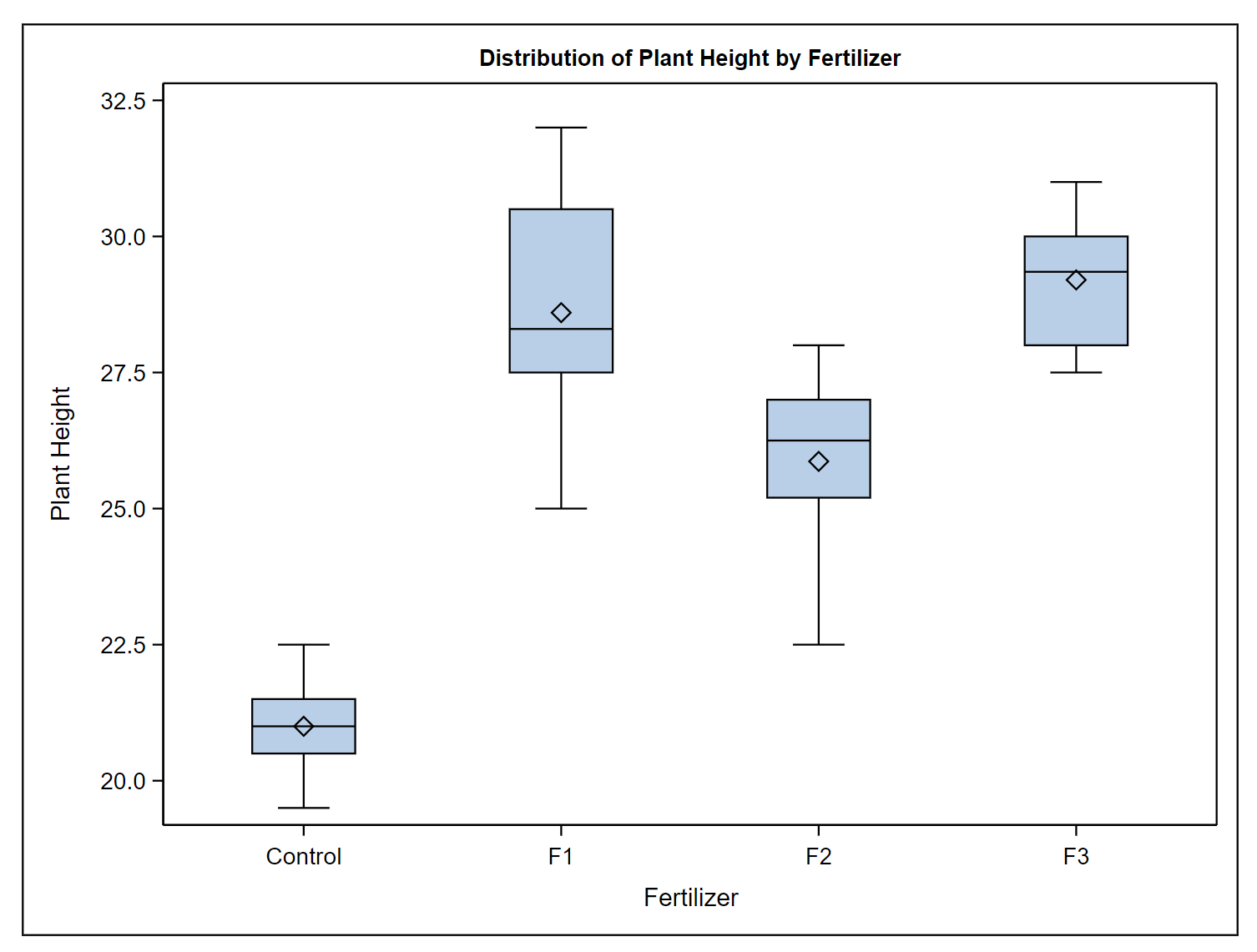
Pictured in the graph below, we can imagine testing three kinds of fertilizer and also one group of plants that are untreated (the control). The plant biologist kept all the plants under controlled conditions in the greenhouse, to focus on the effect of the fertilizer, the only thing we know to differ among the plants. At the end of the experiment, the biologist measured the height of each plant. Plant height is the dependent or response variable and is plotted on the vertical (\(y\)) axis. The biologist used a simple boxplot to plot the difference in the heights.

Box plot showing the distribution of plant height, separated by fertilizer treatment. — Figure \(\PageIndex{1}\): Boxplot of plant height distribution by fertilizer.

This boxplot is a customary way to show treatment (or factor) level differences. In this case, there was only one treatment: fertilizer. The fertilizer treatment had four levels that included the control, which received no fertilizer. Using this language convention is important because later on we will be using ANOVA to handle multi-factor studies (for example if the biologist manipulated the amount of water AND the type of fertilizer) and we will need to be able to refer to different treatments, each with their own set of levels.

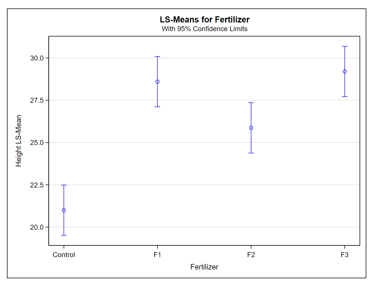
Another alternative for viewing the differences in the heights is with a means plot (a scatter or interval plot):

LS-Means plot for fertilizer treatments, with 95% confidence limits. — Figure \(\PageIndex{2}\): Means plot for fertilizer with 95% confidence limits.

This second method to plot the difference in the means of the treatments provides essentially the same information. However, this plot illustrates the variability in the data with 'error bars' that are the 95% confidence interval limits around the means.

In between the statement of a Working Hypothesis and the creation of the 95% confidence intervals used to create this means plot is a 7-step process of statistical hypothesis testing, presented in the following section.