5.3: Introduction to the z table
- Page ID
- 17338
\( \newcommand{\vecs}[1]{\overset { \scriptstyle \rightharpoonup} {\mathbf{#1}} } \)
\( \newcommand{\vecd}[1]{\overset{-\!-\!\rightharpoonup}{\vphantom{a}\smash {#1}}} \)
\( \newcommand{\dsum}{\displaystyle\sum\limits} \)
\( \newcommand{\dint}{\displaystyle\int\limits} \)
\( \newcommand{\dlim}{\displaystyle\lim\limits} \)
\( \newcommand{\id}{\mathrm{id}}\) \( \newcommand{\Span}{\mathrm{span}}\)
( \newcommand{\kernel}{\mathrm{null}\,}\) \( \newcommand{\range}{\mathrm{range}\,}\)
\( \newcommand{\RealPart}{\mathrm{Re}}\) \( \newcommand{\ImaginaryPart}{\mathrm{Im}}\)
\( \newcommand{\Argument}{\mathrm{Arg}}\) \( \newcommand{\norm}[1]{\| #1 \|}\)
\( \newcommand{\inner}[2]{\langle #1, #2 \rangle}\)
\( \newcommand{\Span}{\mathrm{span}}\)
\( \newcommand{\id}{\mathrm{id}}\)
\( \newcommand{\Span}{\mathrm{span}}\)
\( \newcommand{\kernel}{\mathrm{null}\,}\)
\( \newcommand{\range}{\mathrm{range}\,}\)
\( \newcommand{\RealPart}{\mathrm{Re}}\)
\( \newcommand{\ImaginaryPart}{\mathrm{Im}}\)
\( \newcommand{\Argument}{\mathrm{Arg}}\)
\( \newcommand{\norm}[1]{\| #1 \|}\)
\( \newcommand{\inner}[2]{\langle #1, #2 \rangle}\)
\( \newcommand{\Span}{\mathrm{span}}\) \( \newcommand{\AA}{\unicode[.8,0]{x212B}}\)
\( \newcommand{\vectorA}[1]{\vec{#1}} % arrow\)
\( \newcommand{\vectorAt}[1]{\vec{\text{#1}}} % arrow\)
\( \newcommand{\vectorB}[1]{\overset { \scriptstyle \rightharpoonup} {\mathbf{#1}} } \)
\( \newcommand{\vectorC}[1]{\textbf{#1}} \)
\( \newcommand{\vectorD}[1]{\overrightarrow{#1}} \)
\( \newcommand{\vectorDt}[1]{\overrightarrow{\text{#1}}} \)
\( \newcommand{\vectE}[1]{\overset{-\!-\!\rightharpoonup}{\vphantom{a}\smash{\mathbf {#1}}}} \)
\( \newcommand{\vecs}[1]{\overset { \scriptstyle \rightharpoonup} {\mathbf{#1}} } \)
\(\newcommand{\longvect}{\overrightarrow}\)
\( \newcommand{\vecd}[1]{\overset{-\!-\!\rightharpoonup}{\vphantom{a}\smash {#1}}} \)
\(\newcommand{\avec}{\mathbf a}\) \(\newcommand{\bvec}{\mathbf b}\) \(\newcommand{\cvec}{\mathbf c}\) \(\newcommand{\dvec}{\mathbf d}\) \(\newcommand{\dtil}{\widetilde{\mathbf d}}\) \(\newcommand{\evec}{\mathbf e}\) \(\newcommand{\fvec}{\mathbf f}\) \(\newcommand{\nvec}{\mathbf n}\) \(\newcommand{\pvec}{\mathbf p}\) \(\newcommand{\qvec}{\mathbf q}\) \(\newcommand{\svec}{\mathbf s}\) \(\newcommand{\tvec}{\mathbf t}\) \(\newcommand{\uvec}{\mathbf u}\) \(\newcommand{\vvec}{\mathbf v}\) \(\newcommand{\wvec}{\mathbf w}\) \(\newcommand{\xvec}{\mathbf x}\) \(\newcommand{\yvec}{\mathbf y}\) \(\newcommand{\zvec}{\mathbf z}\) \(\newcommand{\rvec}{\mathbf r}\) \(\newcommand{\mvec}{\mathbf m}\) \(\newcommand{\zerovec}{\mathbf 0}\) \(\newcommand{\onevec}{\mathbf 1}\) \(\newcommand{\real}{\mathbb R}\) \(\newcommand{\twovec}[2]{\left[\begin{array}{r}#1 \\ #2 \end{array}\right]}\) \(\newcommand{\ctwovec}[2]{\left[\begin{array}{c}#1 \\ #2 \end{array}\right]}\) \(\newcommand{\threevec}[3]{\left[\begin{array}{r}#1 \\ #2 \\ #3 \end{array}\right]}\) \(\newcommand{\cthreevec}[3]{\left[\begin{array}{c}#1 \\ #2 \\ #3 \end{array}\right]}\) \(\newcommand{\fourvec}[4]{\left[\begin{array}{r}#1 \\ #2 \\ #3 \\ #4 \end{array}\right]}\) \(\newcommand{\cfourvec}[4]{\left[\begin{array}{c}#1 \\ #2 \\ #3 \\ #4 \end{array}\right]}\) \(\newcommand{\fivevec}[5]{\left[\begin{array}{r}#1 \\ #2 \\ #3 \\ #4 \\ #5 \\ \end{array}\right]}\) \(\newcommand{\cfivevec}[5]{\left[\begin{array}{c}#1 \\ #2 \\ #3 \\ #4 \\ #5 \\ \end{array}\right]}\) \(\newcommand{\mattwo}[4]{\left[\begin{array}{rr}#1 \amp #2 \\ #3 \amp #4 \\ \end{array}\right]}\) \(\newcommand{\laspan}[1]{\text{Span}\{#1\}}\) \(\newcommand{\bcal}{\cal B}\) \(\newcommand{\ccal}{\cal C}\) \(\newcommand{\scal}{\cal S}\) \(\newcommand{\wcal}{\cal W}\) \(\newcommand{\ecal}{\cal E}\) \(\newcommand{\coords}[2]{\left\{#1\right\}_{#2}}\) \(\newcommand{\gray}[1]{\color{gray}{#1}}\) \(\newcommand{\lgray}[1]{\color{lightgray}{#1}}\) \(\newcommand{\rank}{\operatorname{rank}}\) \(\newcommand{\row}{\text{Row}}\) \(\newcommand{\col}{\text{Col}}\) \(\renewcommand{\row}{\text{Row}}\) \(\newcommand{\nul}{\text{Nul}}\) \(\newcommand{\var}{\text{Var}}\) \(\newcommand{\corr}{\text{corr}}\) \(\newcommand{\len}[1]{\left|#1\right|}\) \(\newcommand{\bbar}{\overline{\bvec}}\) \(\newcommand{\bhat}{\widehat{\bvec}}\) \(\newcommand{\bperp}{\bvec^\perp}\) \(\newcommand{\xhat}{\widehat{\xvec}}\) \(\newcommand{\vhat}{\widehat{\vvec}}\) \(\newcommand{\uhat}{\widehat{\uvec}}\) \(\newcommand{\what}{\widehat{\wvec}}\) \(\newcommand{\Sighat}{\widehat{\Sigma}}\) \(\newcommand{\lt}{<}\) \(\newcommand{\gt}{>}\) \(\newcommand{\amp}{&}\) \(\definecolor{fillinmathshade}{gray}{0.9}\)To introduce the table of critical z-scores, we'll first refresh and add to what you learned last chapter about distributions
Probability Distributions and Normal Distributions
Recall that the normal distribution has an area under its curve that is equal to 1 and that it can be split into sections by drawing a line through it that corresponds to standard deviations from the mean. These lines marked specific z-scores. These sections between the marked lines have specific probabilities of scores falling in these areas under the normal curve.
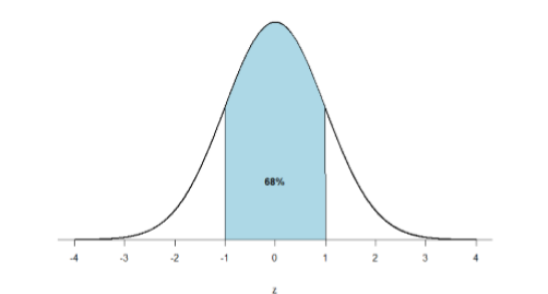
First, let’s look back at the area between \(z\) = -1.00 and \(z\) = 1.00 presented in Figure \(\PageIndex{1}\). We were told earlier that this region contains 68% of the area under the curve. Thus, if we randomly chose a \(z\)-score from all possible z-scores, there is a 68% chance that it will be between \(z = -1.00\) and \(z = 1.00\) (within one standard deviation below and one standard deviation above the mean) because those are the \(z\)-scores that satisfy our criteria.

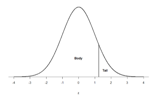
Take a look at the normal distribution in Figure \(\PageIndex{2}\) which has a line drawn through it as \(z\) = 1.25. This line creates two sections of the distribution: the smaller section called the tail and the larger section called the body. Differentiating between the body and the tail does not depend on which side of the distribution the line is drawn. All that matters is the relative size of the pieces: bigger is always body.

We can then find the proportion of the area in the body and tail based on where the line was drawn (i.e. at what \(z\)-score). Mathematically this is done using calculus, but we don't need to know how to do all that! The exact proportions for are given you to you in the Standard Normal Distribution Table, also known at the \(z\)-table. Using the values in this table, we can find the area under the normal curve in any body, tail, or combination of tails no matter which \(z\)-scores are used to define them.
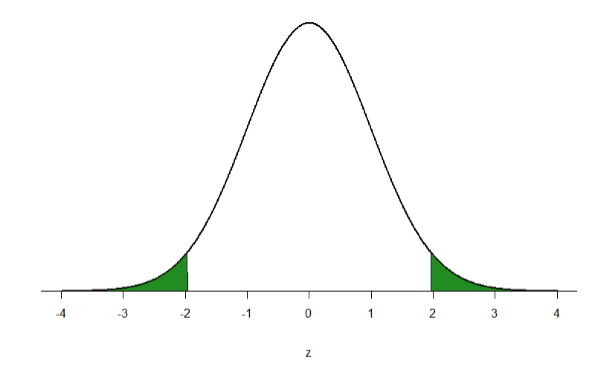
Let’s look at an example: let’s find the area in the tails of the distribution for values less than \(z\) = -1.96 (farther negative and therefore more extreme) and greater than \(z\) = 1.96 (farther positive and therefore more extreme). Dr. Foster didn't just pick this z-score out of nowhere, but we'll get to that later. Let’s find the area corresponding to the region illustrated in Figure \(\PageIndex{3}\), which corresponds to the area more extreme than \(z\) = -1.96 and \(z\) = 1.96.

If we go to the \(z\)-table shown in the Critical Values of z Table page (which can also be found from the Common Critical Value Tables at the end of this book), we will see one column header that has a \(z\), bidirectional arrows, and then \(p\). This means that, for the entire table (all 14ish columns), there are really two columns (or sub-columns. The numbers on the left (starting with -3.00 and ending with 3.00) are z-scores. The numbers on the right (starting with .00135 and ending with .99865) are probabilities (p-values). So, if you multiply the p-values by 100, you get a percentage.
Let’s start with the tail for \(z\) = 1.96. What p-value corresponds to 1.96 from the z-table in Table \(\PageIndex{1}\)?
Example \(\PageIndex{1}\)
What p-value corresponds to 1.96 from the z-table in Table \(\PageIndex{1}\)?
Solution
For z = 1.96, p = .97500
If we multiply that by 100, that means that 97.50% of the scores in this distribution will be below this score. Look at Figure \(\PageIndex{3}\) again. This is saying that 97.5 % of scores are outside of the shaded area on the right. That means that 2.5% of scores in a normal distribution will be higher than this score (100% - 97.50% = 2.50%). In other words, the probability of a raw score being higher than a z-score is p=.025.
If do the same thing with |(z = -1.96|), we find that the p-value for \(z = -1.96\) is .025. That means that \(2.5\%\) of raw scores should be below a z-score of \(-1.96\); according to Figure \(\PageIndex{3}\), that is the shaded area on the left side. What did we just learn? That the shaded areas for the same z-score (negative or positive) are the same p-value, the same probability. We can also find the total probabilities of a score being in the two shaded regions by simply adding the areas together to get 0.0500. Thus, there is a 5% chance of randomly getting a value more extreme than \(z = -1.96\) or \(z = 1.96\) (this particular value and region will become incredibly important later). And, because we know that z-scores are really just standard deviations, this means that it is very unlikely (probability of \(5\%\)) to get a score that is almost two standard deviations away from the mean (\(-1.96\) below the mean or 1.96 above the mean).
Attributions & Contributors
Foster et al. (University of Missouri-St. Louis, Rice University, & University of Houston, Downtown Campus)


