2.8: More Applications
- Page ID
- 26500

\( \newcommand{\vecs}[1]{\overset { \scriptstyle \rightharpoonup} {\mathbf{#1}} } \)
\( \newcommand{\vecd}[1]{\overset{-\!-\!\rightharpoonup}{\vphantom{a}\smash {#1}}} \)
\( \newcommand{\dsum}{\displaystyle\sum\limits} \)
\( \newcommand{\dint}{\displaystyle\int\limits} \)
\( \newcommand{\dlim}{\displaystyle\lim\limits} \)
\( \newcommand{\id}{\mathrm{id}}\) \( \newcommand{\Span}{\mathrm{span}}\)
( \newcommand{\kernel}{\mathrm{null}\,}\) \( \newcommand{\range}{\mathrm{range}\,}\)
\( \newcommand{\RealPart}{\mathrm{Re}}\) \( \newcommand{\ImaginaryPart}{\mathrm{Im}}\)
\( \newcommand{\Argument}{\mathrm{Arg}}\) \( \newcommand{\norm}[1]{\| #1 \|}\)
\( \newcommand{\inner}[2]{\langle #1, #2 \rangle}\)
\( \newcommand{\Span}{\mathrm{span}}\)
\( \newcommand{\id}{\mathrm{id}}\)
\( \newcommand{\Span}{\mathrm{span}}\)
\( \newcommand{\kernel}{\mathrm{null}\,}\)
\( \newcommand{\range}{\mathrm{range}\,}\)
\( \newcommand{\RealPart}{\mathrm{Re}}\)
\( \newcommand{\ImaginaryPart}{\mathrm{Im}}\)
\( \newcommand{\Argument}{\mathrm{Arg}}\)
\( \newcommand{\norm}[1]{\| #1 \|}\)
\( \newcommand{\inner}[2]{\langle #1, #2 \rangle}\)
\( \newcommand{\Span}{\mathrm{span}}\) \( \newcommand{\AA}{\unicode[.8,0]{x212B}}\)
\( \newcommand{\vectorA}[1]{\vec{#1}} % arrow\)
\( \newcommand{\vectorAt}[1]{\vec{\text{#1}}} % arrow\)
\( \newcommand{\vectorB}[1]{\overset { \scriptstyle \rightharpoonup} {\mathbf{#1}} } \)
\( \newcommand{\vectorC}[1]{\textbf{#1}} \)
\( \newcommand{\vectorD}[1]{\overrightarrow{#1}} \)
\( \newcommand{\vectorDt}[1]{\overrightarrow{\text{#1}}} \)
\( \newcommand{\vectE}[1]{\overset{-\!-\!\rightharpoonup}{\vphantom{a}\smash{\mathbf {#1}}}} \)
\( \newcommand{\vecs}[1]{\overset { \scriptstyle \rightharpoonup} {\mathbf{#1}} } \)
\(\newcommand{\longvect}{\overrightarrow}\)
\( \newcommand{\vecd}[1]{\overset{-\!-\!\rightharpoonup}{\vphantom{a}\smash {#1}}} \)
\(\newcommand{\avec}{\mathbf a}\) \(\newcommand{\bvec}{\mathbf b}\) \(\newcommand{\cvec}{\mathbf c}\) \(\newcommand{\dvec}{\mathbf d}\) \(\newcommand{\dtil}{\widetilde{\mathbf d}}\) \(\newcommand{\evec}{\mathbf e}\) \(\newcommand{\fvec}{\mathbf f}\) \(\newcommand{\nvec}{\mathbf n}\) \(\newcommand{\pvec}{\mathbf p}\) \(\newcommand{\qvec}{\mathbf q}\) \(\newcommand{\svec}{\mathbf s}\) \(\newcommand{\tvec}{\mathbf t}\) \(\newcommand{\uvec}{\mathbf u}\) \(\newcommand{\vvec}{\mathbf v}\) \(\newcommand{\wvec}{\mathbf w}\) \(\newcommand{\xvec}{\mathbf x}\) \(\newcommand{\yvec}{\mathbf y}\) \(\newcommand{\zvec}{\mathbf z}\) \(\newcommand{\rvec}{\mathbf r}\) \(\newcommand{\mvec}{\mathbf m}\) \(\newcommand{\zerovec}{\mathbf 0}\) \(\newcommand{\onevec}{\mathbf 1}\) \(\newcommand{\real}{\mathbb R}\) \(\newcommand{\twovec}[2]{\left[\begin{array}{r}#1 \\ #2 \end{array}\right]}\) \(\newcommand{\ctwovec}[2]{\left[\begin{array}{c}#1 \\ #2 \end{array}\right]}\) \(\newcommand{\threevec}[3]{\left[\begin{array}{r}#1 \\ #2 \\ #3 \end{array}\right]}\) \(\newcommand{\cthreevec}[3]{\left[\begin{array}{c}#1 \\ #2 \\ #3 \end{array}\right]}\) \(\newcommand{\fourvec}[4]{\left[\begin{array}{r}#1 \\ #2 \\ #3 \\ #4 \end{array}\right]}\) \(\newcommand{\cfourvec}[4]{\left[\begin{array}{c}#1 \\ #2 \\ #3 \\ #4 \end{array}\right]}\) \(\newcommand{\fivevec}[5]{\left[\begin{array}{r}#1 \\ #2 \\ #3 \\ #4 \\ #5 \\ \end{array}\right]}\) \(\newcommand{\cfivevec}[5]{\left[\begin{array}{c}#1 \\ #2 \\ #3 \\ #4 \\ #5 \\ \end{array}\right]}\) \(\newcommand{\mattwo}[4]{\left[\begin{array}{rr}#1 \amp #2 \\ #3 \amp #4 \\ \end{array}\right]}\) \(\newcommand{\laspan}[1]{\text{Span}\{#1\}}\) \(\newcommand{\bcal}{\cal B}\) \(\newcommand{\ccal}{\cal C}\) \(\newcommand{\scal}{\cal S}\) \(\newcommand{\wcal}{\cal W}\) \(\newcommand{\ecal}{\cal E}\) \(\newcommand{\coords}[2]{\left\{#1\right\}_{#2}}\) \(\newcommand{\gray}[1]{\color{gray}{#1}}\) \(\newcommand{\lgray}[1]{\color{lightgray}{#1}}\) \(\newcommand{\rank}{\operatorname{rank}}\) \(\newcommand{\row}{\text{Row}}\) \(\newcommand{\col}{\text{Col}}\) \(\renewcommand{\row}{\text{Row}}\) \(\newcommand{\nul}{\text{Nul}}\) \(\newcommand{\var}{\text{Var}}\) \(\newcommand{\corr}{\text{corr}}\) \(\newcommand{\len}[1]{\left|#1\right|}\) \(\newcommand{\bbar}{\overline{\bvec}}\) \(\newcommand{\bhat}{\widehat{\bvec}}\) \(\newcommand{\bperp}{\bvec^\perp}\) \(\newcommand{\xhat}{\widehat{\xvec}}\) \(\newcommand{\vhat}{\widehat{\vvec}}\) \(\newcommand{\uhat}{\widehat{\uvec}}\) \(\newcommand{\what}{\widehat{\wvec}}\) \(\newcommand{\Sighat}{\widehat{\Sigma}}\) \(\newcommand{\lt}{<}\) \(\newcommand{\gt}{>}\) \(\newcommand{\amp}{&}\) \(\definecolor{fillinmathshade}{gray}{0.9}\)In this section, you will learn to:
- Solve a linear system in two variables.
- Find the equilibrium point when a demand and a supply equation are given.
- Find the break-even point when the revenue and the cost functions are given.
Finding the Point of Intersection of Two Lines
In this section, we will do application problems that involve the intersection of lines. Therefore, before we proceed any further, we will first learn how to find the intersection of two lines.
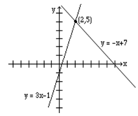
Find the intersection of the line \(y = 3x -1\) and the line \(y = - x + 7\).
Solution
We graph both lines on the same axes, as shown below, and read the solution (2, 5).
Finding an intersection of two lines graphically is not always easy or practical; therefore, we will now learn to solve these problems algebraically.
At the point where two lines intersect, the \(x\) and \(y\) values for both lines are the same. So in order to find the intersection, we either let the \(x\)-values or the \(y\)-values equal.
If we were to solve the above example algebraically, it will be easier to let the y-values equal. Since \(y = 3x - 1\) for the first line, and \(y = - x + 7\) for the second line, by letting the y-values equal, we get
\begin{aligned}
3 x-1&=-x+7\\
4 x&=8\\
x&=2
\end{aligned}
By substituting \(x = 2\) in any of the two equations, we obtain \(y = 5\).
Hence, the solution (2, 5).
A common algebraic method used to solve systems of equations is called the elimination method. The object is to eliminate one of the two variables by adding the left and right sides of the equations together. Once one variable is eliminated, we have an equation with only one variable for can be solved. Finally, by substituting the value of the variable that has been found in one of the original equations, we get the value of the other variable.
Find the intersection of the lines \(2x + y = 7\) and \(3x - y = 3\) by the elimination method.
Solution
We add the left and right sides of the two equations.
\begin{aligned}
2 x+y&=7\\
3x-y&=3 \\ \hline 5x&=10\\
x&=2
\end{aligned}
Now we substitute \(x = 2\) in any of the two equations and solve for \(y\).
\begin{aligned}
2(2)+y&=7\\
y&=3
\end{aligned}
Therefore, the solution is (2, 3).
Solve the system of equations \(x + 2y = 3\) and \(2x + 3y = 4\) by the elimination method.
Solution
If we add the two equations, none of the variables are eliminated. But the variable \(x\) can be eliminated by multiplying the first equation by -2, and leaving the second equation unchanged.
\begin{aligned}
-2 x-4 y &=-6 \\
2 x+3 y &=4 \\
\hline -y &=-2 \\
y &=2
\end{aligned}
Substituting \(y = 2\) in \(x + 2y = 3\), we get
\begin{array}{l}
x+2(2)=3 \\
x=-1
\end{array}
Therefore, the solution is (-1, 2).
Solve the system of equations \(3x - 4y = 5\) and \(4x - 5y = 6\).
Solution
This time, we multiply the first equation by - 4 and the second by 3 before adding. (The choice of numbers is not unique.)
\begin{aligned}
-12 x+16 y &=-20 \\
12 x-15 y &=18 \\ \hline y&=-2
\end{aligned}
By substituting y = - 2 in any one of the equations, we get x = -1.
Hence the solution is (-1, -2).
SUPPLY, DEMAND AND THE EQUILIBRIUM MARKET PRICE
In a free market economy the supply curve for a commodity is the number of items of a product that can be made available at different prices, and the demand curve is the number of items the consumer will buy at different prices.
As the price of a product increases, its demand decreases and supply increases. On the other hand, as the price decreases the demand increases and supply decreases. The equilibrium price is reached when the demand equals the supply.
The supply curve for a product is \(y = 3.5x - 14\) and the demand curve for the same product is \(y = - 2.5x + 34\), where x is the price and y the number of items produced. Find the following.
- How many items will be supplied at a price of $10?
- How many items will be demanded at a price of $10?
- Determine the equilibrium price.
- How many items will be produced at the equilibrium price?
Solution
a) We substitute \(x = 10\) in the supply equation, \(y = 3.5x - 14\); the answer is \(y = 3.5(10) - 14 =21\).
b) We substitute \(x = 10\) in the demand equation, \(y = - 2.5x + 34\); the answer is \(y = - 2.5(10) + 34= 9\).
c) By letting the supply equal the demand, we get
\begin{aligned}
3.5x-14 &=-25x+34 \\
6x &=48 \\
x &=\$8
\end{aligned}
d) We substitute \(x = 8\) in either the supply or the demand equation; we get \(y = 14\).

The graph shows the intersection of the supply and the demand functions and their point of intersection, (8,14).
Interpretation: At equilibrium, the price is $8 per item, and 14 items are produced by suppliers and purchased by consumers.
The Break-Even Point
In a business, the profit is generated by selling products.
- If a company sells x number of items at a price P, then the revenue R is the price multiplied by number of items sold: \(R = P \cdot x\).
- The production costs C are the sum of the variable costs and the fixed costs, and are often written as C = mx + b, where x is the number of items manufactured.
-
- The slope m is the called marginal cost and represents the cost to produce one additional item or unit.
- The variable cost, mx, depends on how much is being produced
- The fixed cost b is constant; it does not change no matter how much is produced.
- Profit is equal to Revenue minus Cost: Profit = R − C
A company makes a profit if the revenue is greater than the cost. There is a loss if the cost is greater than the revenue. The point on the graph where the revenue equals the cost is called the break-even point. At the break-even point, profit is 0.
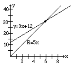
If the revenue function of a product is \(R = 5x\) and the cost function is \(y = 3x + 12\), find the following.
- If 4 items are produced, what will the revenue be?
- What is the cost of producing 4 items?
- How many items should be produced to break even?
- What will be the revenue and the cost at the break-even point?
Solution
a) We substitute \(x = 4\) in the revenue equation \(R = 5x\), and the answer is \(R = 20\).
b) We substitute \(x = 4\) in the cost equation \(C = 3x + 12\), and the answer is \(C = 24\).
c) By letting the revenue equal the cost, we get
\begin{aligned}
5x&=3x+12 \\
x&=6 \\
\end{aligned}
d) Substitute \(x = 6\) in either the revenue or the cost equation: we get \(R = C = 30\).
The graph below shows the intersection of the revenue and cost functions and their point of intersection, (6, 30).