2.5: Absolute Value Equations
- Page ID
- 26496
\( \newcommand{\vecs}[1]{\overset { \scriptstyle \rightharpoonup} {\mathbf{#1}} } \)
\( \newcommand{\vecd}[1]{\overset{-\!-\!\rightharpoonup}{\vphantom{a}\smash {#1}}} \)
\( \newcommand{\dsum}{\displaystyle\sum\limits} \)
\( \newcommand{\dint}{\displaystyle\int\limits} \)
\( \newcommand{\dlim}{\displaystyle\lim\limits} \)
\( \newcommand{\id}{\mathrm{id}}\) \( \newcommand{\Span}{\mathrm{span}}\)
( \newcommand{\kernel}{\mathrm{null}\,}\) \( \newcommand{\range}{\mathrm{range}\,}\)
\( \newcommand{\RealPart}{\mathrm{Re}}\) \( \newcommand{\ImaginaryPart}{\mathrm{Im}}\)
\( \newcommand{\Argument}{\mathrm{Arg}}\) \( \newcommand{\norm}[1]{\| #1 \|}\)
\( \newcommand{\inner}[2]{\langle #1, #2 \rangle}\)
\( \newcommand{\Span}{\mathrm{span}}\)
\( \newcommand{\id}{\mathrm{id}}\)
\( \newcommand{\Span}{\mathrm{span}}\)
\( \newcommand{\kernel}{\mathrm{null}\,}\)
\( \newcommand{\range}{\mathrm{range}\,}\)
\( \newcommand{\RealPart}{\mathrm{Re}}\)
\( \newcommand{\ImaginaryPart}{\mathrm{Im}}\)
\( \newcommand{\Argument}{\mathrm{Arg}}\)
\( \newcommand{\norm}[1]{\| #1 \|}\)
\( \newcommand{\inner}[2]{\langle #1, #2 \rangle}\)
\( \newcommand{\Span}{\mathrm{span}}\) \( \newcommand{\AA}{\unicode[.8,0]{x212B}}\)
\( \newcommand{\vectorA}[1]{\vec{#1}} % arrow\)
\( \newcommand{\vectorAt}[1]{\vec{\text{#1}}} % arrow\)
\( \newcommand{\vectorB}[1]{\overset { \scriptstyle \rightharpoonup} {\mathbf{#1}} } \)
\( \newcommand{\vectorC}[1]{\textbf{#1}} \)
\( \newcommand{\vectorD}[1]{\overrightarrow{#1}} \)
\( \newcommand{\vectorDt}[1]{\overrightarrow{\text{#1}}} \)
\( \newcommand{\vectE}[1]{\overset{-\!-\!\rightharpoonup}{\vphantom{a}\smash{\mathbf {#1}}}} \)
\( \newcommand{\vecs}[1]{\overset { \scriptstyle \rightharpoonup} {\mathbf{#1}} } \)
\(\newcommand{\longvect}{\overrightarrow}\)
\( \newcommand{\vecd}[1]{\overset{-\!-\!\rightharpoonup}{\vphantom{a}\smash {#1}}} \)
\(\newcommand{\avec}{\mathbf a}\) \(\newcommand{\bvec}{\mathbf b}\) \(\newcommand{\cvec}{\mathbf c}\) \(\newcommand{\dvec}{\mathbf d}\) \(\newcommand{\dtil}{\widetilde{\mathbf d}}\) \(\newcommand{\evec}{\mathbf e}\) \(\newcommand{\fvec}{\mathbf f}\) \(\newcommand{\nvec}{\mathbf n}\) \(\newcommand{\pvec}{\mathbf p}\) \(\newcommand{\qvec}{\mathbf q}\) \(\newcommand{\svec}{\mathbf s}\) \(\newcommand{\tvec}{\mathbf t}\) \(\newcommand{\uvec}{\mathbf u}\) \(\newcommand{\vvec}{\mathbf v}\) \(\newcommand{\wvec}{\mathbf w}\) \(\newcommand{\xvec}{\mathbf x}\) \(\newcommand{\yvec}{\mathbf y}\) \(\newcommand{\zvec}{\mathbf z}\) \(\newcommand{\rvec}{\mathbf r}\) \(\newcommand{\mvec}{\mathbf m}\) \(\newcommand{\zerovec}{\mathbf 0}\) \(\newcommand{\onevec}{\mathbf 1}\) \(\newcommand{\real}{\mathbb R}\) \(\newcommand{\twovec}[2]{\left[\begin{array}{r}#1 \\ #2 \end{array}\right]}\) \(\newcommand{\ctwovec}[2]{\left[\begin{array}{c}#1 \\ #2 \end{array}\right]}\) \(\newcommand{\threevec}[3]{\left[\begin{array}{r}#1 \\ #2 \\ #3 \end{array}\right]}\) \(\newcommand{\cthreevec}[3]{\left[\begin{array}{c}#1 \\ #2 \\ #3 \end{array}\right]}\) \(\newcommand{\fourvec}[4]{\left[\begin{array}{r}#1 \\ #2 \\ #3 \\ #4 \end{array}\right]}\) \(\newcommand{\cfourvec}[4]{\left[\begin{array}{c}#1 \\ #2 \\ #3 \\ #4 \end{array}\right]}\) \(\newcommand{\fivevec}[5]{\left[\begin{array}{r}#1 \\ #2 \\ #3 \\ #4 \\ #5 \\ \end{array}\right]}\) \(\newcommand{\cfivevec}[5]{\left[\begin{array}{c}#1 \\ #2 \\ #3 \\ #4 \\ #5 \\ \end{array}\right]}\) \(\newcommand{\mattwo}[4]{\left[\begin{array}{rr}#1 \amp #2 \\ #3 \amp #4 \\ \end{array}\right]}\) \(\newcommand{\laspan}[1]{\text{Span}\{#1\}}\) \(\newcommand{\bcal}{\cal B}\) \(\newcommand{\ccal}{\cal C}\) \(\newcommand{\scal}{\cal S}\) \(\newcommand{\wcal}{\cal W}\) \(\newcommand{\ecal}{\cal E}\) \(\newcommand{\coords}[2]{\left\{#1\right\}_{#2}}\) \(\newcommand{\gray}[1]{\color{gray}{#1}}\) \(\newcommand{\lgray}[1]{\color{lightgray}{#1}}\) \(\newcommand{\rank}{\operatorname{rank}}\) \(\newcommand{\row}{\text{Row}}\) \(\newcommand{\col}{\text{Col}}\) \(\renewcommand{\row}{\text{Row}}\) \(\newcommand{\nul}{\text{Nul}}\) \(\newcommand{\var}{\text{Var}}\) \(\newcommand{\corr}{\text{corr}}\) \(\newcommand{\len}[1]{\left|#1\right|}\) \(\newcommand{\bbar}{\overline{\bvec}}\) \(\newcommand{\bhat}{\widehat{\bvec}}\) \(\newcommand{\bperp}{\bvec^\perp}\) \(\newcommand{\xhat}{\widehat{\xvec}}\) \(\newcommand{\vhat}{\widehat{\vvec}}\) \(\newcommand{\uhat}{\widehat{\uvec}}\) \(\newcommand{\what}{\widehat{\wvec}}\) \(\newcommand{\Sighat}{\widehat{\Sigma}}\) \(\newcommand{\lt}{<}\) \(\newcommand{\gt}{>}\) \(\newcommand{\amp}{&}\) \(\definecolor{fillinmathshade}{gray}{0.9}\)In the previous section, we defined
\[|x|=\left\{\begin{array}{ll}{-x,} & {\text { if } x<0} \\ {x,} & {\text { if } x \geq 0}\end{array}\right. \nonumber \]
and we saw that the graph of the absolute value function defined by f(x) = |x| has the “V-shape” shown in Figure \(\PageIndex{1}\).
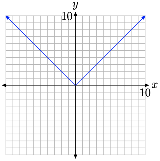 Figure \(\PageIndex{1}\). The graph of the absolute value function f(x) = |x|.
It is important to note that the equation of the left-hand branch of the “V” is y = −x. Typical points on this branch are (−1, 1), (−2, 2), (−3, 3), etc. It is equally important to note that the right-hand branch of the “V” has equation y = x. Typical points on this branch are (1, 1), (2, 2), (3, 3), etc.
Solving |x| = a
We will now discuss the solutions of the equation
\[|x|=a \nonumber \]
There are three distinct cases to discuss, each of which depends upon the value and sign of the number a.
- Case I: a < 0
If a < 0, then the graph of y = a is a horizontal line that lies strictly below the x-axis, as shown in Figure \(\PageIndex{2}\)(a). In this case, the equation |x| = a has no solutions because the graphs of y = a and y = |x| do not intersect.
- Case II: a = 0
If a = 0, then the graph of y = 0 is a horizontal line that coincides with the x-axis, as shown in Figure \(\PageIndex{2}\)(b). In this case, the equation |x| = 0 has the single solution x = 0, because the horizontal line y = 0 intersects the graph of y = |x| at exactly one point, at x = 0.
- Case III: a > 0
If a > 0, then the graph of y = a is a horizontal line that lies strictly above the x-axis, as shown in Figure \(\PageIndex{2}\)(c). In this case, the equation |x| = a has two solutions, because the graphs of y = a and y = |x| have two points of intersection.
Recall that the left-hand branch of y = |x| has equation y = −x, and points on this branch have the form (−1, 1), (−2, 2), etc. Because the point where the graph of y = a intersects the left-hand branch of y = |x| has y-coordinate y = a, the x-coordinate of this point of intersection is x = −a. This is one solution of |x| = a.
Recall that the right-hand branch of y = |x| has equation y = x, and points on this branch have the form (1, 1), (2, 2), etc. Because the point where the graph of y = a intersects the right-hand branch of y = |x| has y-coordinate y = a, the x-coordinate of this point of intersection is x = a. This is the second solution of |x| = a.
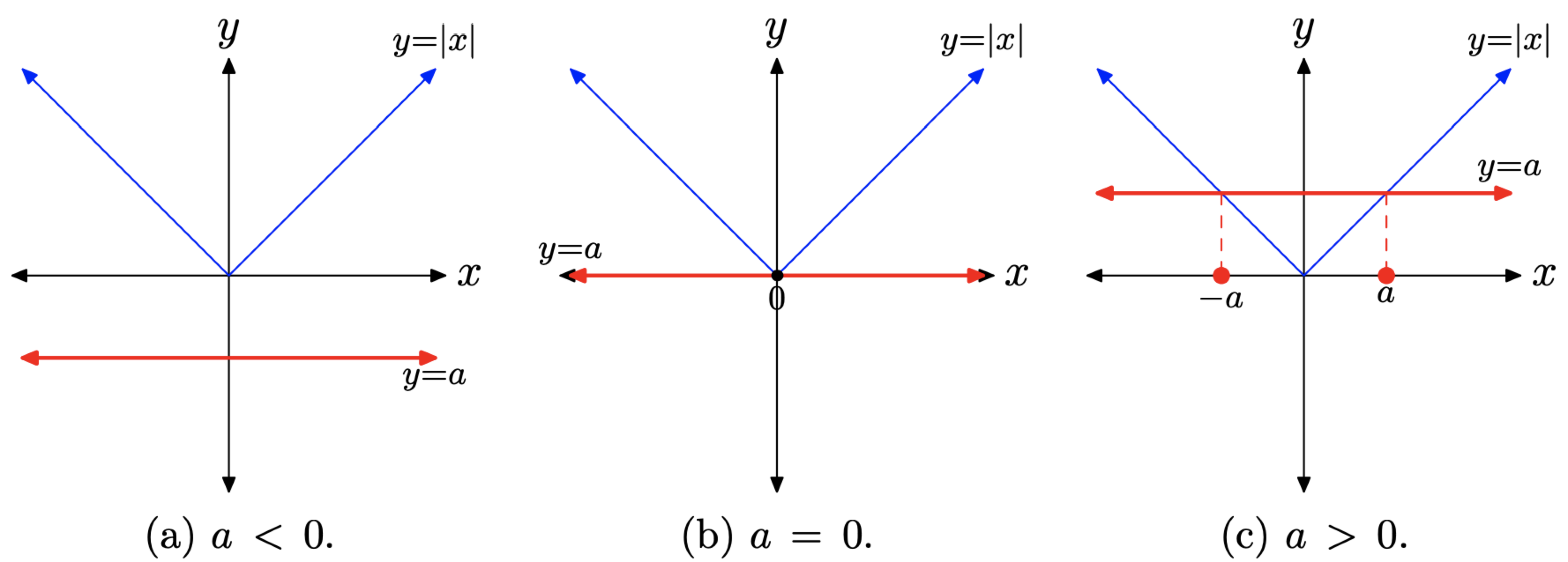 Figure \(\PageIndex{2}\). The solution of |x| = a has three cases.
This discussion leads to the following key result.
The solution of |x| = a depends upon the value and sign of a.
- Case I: a < 0
The equation |x| = a has no solutions.
- Case II: a = 0
The equation |x| = 0 has one solution, x = 0.
- Case III: a > 0
The equation |x| = a has two solutions, x = −a or x = a.
Let’s look at some examples.
Solve |x| = −3 for x.
Solution
The graph of the left-hand side of |x| = −3 is the “V” of Figure \(\PageIndex{2}\)(a). The graph of the right-hand side of |x| = −3 is a horizontal line three units below the x-axis. This has the form of the sketch in Figure \(\PageIndex{2}\)(a). The graphs do not intersect. Therefore, the equation |x| = −3 has no solutions.
An alternate approach is to consider the fact that the absolute value of x can never equal −3. The absolute value of a number is always nonnegative (either zero or positive). Hence, the equation |x| = −3 has no solutions.
Solve |x| = 0 for x
Solution
This is the case shown in Figure \(\PageIndex{2}\)(b). The graph of the left-hand side of |x| = 0 intersects the graph of the right-hand side of |x| = 0 at x = 0. Thus, the only solution of |x| = 0 is x = 0.
Thinking about this algebraically instead of graphically, we know that 0 = 0, but there is no other number with an absolute value of zero. So, intuitively, the only solution of |x| = 0 is x = 0.
Solve |x| = 4 for x.
Solution
The graph of the left-hand side of |x| = 4 is the “V” of Figure \(\PageIndex{2}\)(c). The graph of the right-hand side is a horizontal line 4 units above the x-axis. This has the form of the sketch in Figure \(\PageIndex{2}\)(c). The graphs intersect at (−4, 4) and (4, 4). Therefore, the solutions of |x| = 4 are x = −4 or x = 4.
Alternatively, | − 4| = 4 and |4| = 4, but no other real numbers have absolute value equal to 4. Hence, the only solutions of |x| = 4 are x = −4 or x = 4.
Solve the equation |3 − 2x| = −8 for x.
Solution
If the equation were |x| = −8, we would not hesitate. The equation |x| = −8 has no solutions. However, the reasoning applied to the simple case |x| = −8 works equally well with the equation |3 − 2x| = −8. The left-hand side of this equation must be nonnegative, so its graph must lie above or on the x-axis. The right-hand side of |3−2x| = −8 is a horizontal line 8 units below the x-axis. The graphs cannot intersect, so there is no solution.
We can verify this argument with the graphing calculator. Load the left and righthand sides of |3 − 2x| = −8 into Y1 and Y2, respectively, as shown in Figure \(\PageIndex{3}\)(a). Push the MATH button on your calculator, then right-arrow to the NUM menu, as shown in Figure \(\PageIndex{3}\)(b). Use 1:abs( to enter the absolute value shown in Y1 in Figure \(\PageIndex{3}\)(a). From the ZOOM menu, select 6:ZStandard to produce the image shown in Figure \(\PageIndex{3}\)(c).
Note, that as predicted above, the graph of y = |3 − 2x| lies on or above the xaxis and the graph of y = −8 lies strictly below the x-axis. Hence, the graphs cannot intersect and the equation |3 − 2x| = −8 has no solutions.
 Figure \(\PageIndex{3}\). Using the graphing calculator to examine the solution of |3 − 2x| = −8.
Alternatively, we can provide a completely intuitive solution of |3 − 2x| = −8 by arguing that the left-hand side of this equation is nonnegative, but the right-hand side is negative. This is an impossible situation. Hence, the equation has no solutions.
Solve the equation |3 − 2x| = 0 for x.
Solution
We have argued that the only solution of |x| = 0 is x = 0. Similar reasoning points out that |3 − 2x| = 0 only when 3 − 2x = 0. We solve this equation independently.
\[\begin{aligned} 3-2 x &=0 \\-2 x &=-3 \\ x &=\frac{3}{2} \end{aligned} \nonumber \]
Thus, the only solution of |3 − 2x| = 0 is x = 3/2.
It is worth pointing out that the “tip” or “vertex” of the “V” in Figure \(\PageIndex{3}\)(c) is located at x = 3/2. This is the only location where the graphs of y = |3 − 2x| and y = 0 intersect.
Solve the equation |3 − 2x| = 6 for x.
Solution
In this example, the graph of y = 6 is a horizontal line that lies 6 units above the x-axis, and the graph of y = |3 − 2x| intersects the graph of y = 6 in two locations. You can use the intersect utility to find the points of intersection of the graphs, as we have in Figure \(\PageIndex{4}\)(b) and (c).
 Figure \(\PageIndex{4}\). Using the graphing calculator to find two solutions of |3 − 2x| = 6.
We need a way of summarizing this graphing calculator approach on our homework paper. First, draw a reasonable facsimile of your calculator’s viewing window on your homework paper. Use a ruler to draw all lines. Complete the following checklist.
- Label each axis, in this case with x and y.
- Scale each axis. To do this, press the WINDOW button on your calculator, then report the values of xmin, xmax, ymin, and ymax on the appropriate axis.
- Label each graph with its equation.
- Drop dashed vertical lines from the points of intersection to the x-axis. Shade and label these solutions of the equation on the x-axis.
Following the guidelines in the above checklist, we obtain the image in Figure \(\PageIndex{5}\).
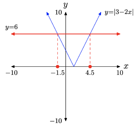 Figure \(\PageIndex{5}\). Reporting a graphical solution of |3 − 2x| = 6.
Algebraic Approach. One can also use an algebraic technique to find the two solutions of |3 − 2x| = 6. Much as |x| = 6 has solutions x = −6 or x = 6, the equation
\[|3-2 x|=6 \nonumber \]
is possible only if the expression inside the absolute values is either equal to −6 or 6. Therefore, write
\[3-2 x=-6 \qquad \text { or } \qquad 3-2 x=6 \nonumber \]
and solve these equations independently
\[\begin{array}{rlrrrl}{3-2 x}&{=}&{-6} & {\text { or }} & {3-2 x}&{=}&{6} \\ {-2 x}&{=}&{-9} && {-2 x}&{=}&{3} \\ {x}&{=}&{\frac{9}{2}} && {x}&{=}&{-\frac{3}{2}}\end{array} \nonumber \]
Because −3/2 = −1.5 and 9/2 = 4.5, these exact solutions agree exactly with the graphical solutions in Figure \(\PageIndex{4}\)(b) and (c).
Let’s summarize the technique involved in solving this important case.
Solving |expression| = a, when a > 0. To solve the equation
\[| \text { expression } |=a, \quad \text { when } a>0 \nonumber \]
set
\[\text { expression }=-a \qquad \text { or } \qquad \text { expression }=a \nonumber \]
then solve each of these equations independently.
For example:
• To solve |2x + 7| = 5, set \[2x + 7 = −5 \qquad or \qquad 2x + 7 = 5 \nonumber \], then solve each of these equations independently.
• To solve |3 − 5x| = 9, set \[3 − 5x = −9 \qquad or \qquad 3 − 5x = 9 \nonumber \], then solve each of these equations independently.
• Note that this technique should not be applied to the equation |2x + 11| = −10, because the right-hand side of the equation is not a positive number. Indeed, in this case, no values of x will make the left-hand side of this equation equal to −10, so the equation has no solutions.
Sometimes we have to do a little algebra before removing the absolute value bars.
Solve the equation \[|x+2|+3=8 \nonumber \] for x.
Solution
First, subtract 3 from both sides of the equation. \[\begin{aligned}|x+2|+3 &=8 \\|x+2|+3-3 &=8-3 \end{aligned} \nonumber \]
This simplifies to \[|x+2|=5 \nonumber \]
Now, either \[x+2=-5 \qquad \text { or } \qquad x+2=5 \nonumber \]
each of which can be solved separately.
\[\begin{array}{rrlrrl}{x+2} & {=} & {-5} & {\text { or }} & {x+2} & {=} & {5} \\ {x+2-2} & {=} & {-5-2} && {x+2-2} & {=} & {5-2} \\ {x} & {=} & {-7} && {x} & {=} & {3}\end{array} \nonumber \]
Solve the equation \[3|x-5|=6 \nonumber \] for x.
Solution
First, divide both sides of the equation by 3
\[\begin{aligned} 3|x-5| &=6 \\ \frac{3|x-5|}{3} &=\frac{6}{3} \end{aligned} \nonumber \]
This simplifies to \[|x-5|=2 \nonumber \]
Now, either \[x-5=-2 \qquad \text { or } \qquad x-5=2 \nonumber \]
each of which can be solved separately.
\[\begin{array}{rllrrl}{x-5} & {=} & {-2} & {\text { or }} & {x-5} & {=} & {2} \\ {x-5+5} & {=} & {-2+5} && {x-5+5} & {=} & {2+5} \\ {x} & {=} & {3} && {x} & {=} & {7}\end{array} \nonumber \]
Properties of Absolute Value
An example will motivate the need for some discussion of the properties of absolute value.
Solve the equation \[\left|\frac{x}{2}-\frac{1}{3}\right|=\frac{1}{4} \nonumber \] for x.
Solution
It is tempting to multiply both sides of this equation by a common denominator as follows.
\[\begin{array}{l}{\left|\dfrac{x}{2}-\dfrac{1}{3}\right|=\dfrac{1}{4}} \\ {12\left|\dfrac{x}{2}-\dfrac{1}{3}\right|=12\left(\dfrac{1}{4}\right)}\end{array} \nonumber \]
If it is permissible to move the 12 inside the absolute values, then we could proceed as follows.
\[\begin{aligned}\left|12\left(\frac{x}{2}-\frac{1}{3}\right)\right| &=3 \\|6 x-4| &=3 \end{aligned} \nonumber \]
Assuming for the moment that this last move is allowable, either
\[6 x-4=-3 \qquad \text { or } \qquad 6 x-4=3 \nonumber \]
Each of these can be solved separately, first by adding 4 to both sides of the equations, then dividing by 6.
\[\begin{array}{rllrrl}{6 x-4} & {=} & {-3} & {\text { or }} & {6 x-4} & {=} & {3} \\ {6 x} & {=} & {1} & &{6 x} & {=} & {7} \\ {x} & {=} & {1 / 6} && {x} & {=} & {7 / 6}\end{array} \nonumber \]
As we’ve used a somewhat questionable move in obtaining these solutions, it would be wise to check our results. First, substitute x = 1/6 into the original equation.
\[\begin{aligned}\left|\frac{x}{2}-\frac{1}{3}\right| &=\frac{1}{4} \\\left|\frac{1 / 6}{2}-\frac{1}{3}\right| &=\frac{1}{4} \\\left|\frac{1}{12}-\frac{1}{3}\right| &=\frac{1}{4} \end{aligned} \nonumber \]
Write equivalent fractions with a common denominator and subtract.
\[\begin{aligned}\left|\frac{1}{12}-\frac{4}{12}\right| &=\frac{1}{4} \\\left|-\frac{3}{12}\right| &=\frac{1}{4} \\\left|-\frac{1}{4}\right| &=\frac{1}{4} \end{aligned} \nonumber \]
Clearly, x = 1/6 checks. We’ll leave the check of the second solution to our readers.
Well, we’ve checked our solutions and they are correct, so it must be the case that
\[12\left|\frac{x}{2}-\frac{1}{3}\right|=\left|12\left(\frac{x}{2}-\frac{1}{3}\right)\right| \nonumber \]
But why? After all, absolute value bars, though they do act as grouping symbols, have a bit more restrictive meaning than ordinary grouping symbols such as parentheses, brackets, and braces.
We state the first property of absolute values.
If a and b are any real numbers, then
\[|a b|=|a||b| \nonumber \]
We can demonstrate the validity of this property by simply checking cases.
- If a and b are both positive real numbers, then so is ab and \(|a||b|=a b\). On the other hand, \(|a||b|=a b\). Thus, \(|ab| = |a||b|\).
- If a and b are both negative real numbers, then ab is positive and \(|ab| = ab\). On the other hand, \(|a||b| = (−a)(−b) = ab\). Thus, \(|ab| = |a||b|\).
We will leave the proof of the remaining two cases as exercises. We can use \(|a||b| = |ab|\) to demonstrate that
\[12\left|\frac{x}{2}-\frac{1}{3}\right|=|12|\left|\frac{x}{2}-\frac{1}{3}\right|=\left|12\left(\frac{x}{2}-\frac{1}{3}\right)\right| \nonumber \]
This validates the method of attack we used to solve equation (12) in Example \(\PageIndex{9}\).
On the other hand, it is not permissible to multiply by a negative number and simply slide the negative number inside the absolute value bars. For example,
\[-2|x-3|=|-2(x-3)| \nonumber \]
is clearly an error (well, it does work for x = 3). For any x except 3, the lefthand side of this result is a negative number, but the right-hand side is a positive number. They are clearly not equal.
In similar fashion, one can demonstrate a second useful property involving absolute value.
If a and b are any real numbers, then \[\left|\frac{a}{b}\right|=\frac{|a|}{|b|} \nonumber \] provided, of course, that \(b \neq 0\).
Again, this can be proved by checking four cases. For example, if a is a positive real number and b is a negative real number, then a/b is negative and \(|a/b| = −a/b\). On the other hand, \(|a|/|b| = a/(−b) = −a/b\).
We leave the proof of the remaining three cases as exercises.
This property is useful in certain situations. For example, should you desire to divide \(|2x − 4|\) by 2, you would proceed as follows.
\[\frac{|2 x-4|}{2}=\frac{|2 x-4|}{|2|}=\left|\frac{2 x-4}{2}\right|=|x-2| \nonumber \]
This technique is useful in several situations. For example, should you want to solve the equation \(|2x − 4| = 6\), you could divide both sides by 2 and apply the quotient property of absolute values.
Distance Revisited
Recall that for any real number x, the absolute value of x is defined as the distance between the real number x and the origin on the real line. In this section, we will push this distance concept a bit further.
Suppose that you have two real numbers on the real line. For example, in the figure that follows, we’ve located 3 and −2 on the real line.

You can determine the distance between the two points by subtracting the number on the left from the number on the right. That is, the distance between the two points is d = 3 − (−2) = 5 units. If you subtract in the other direction, you get the negative of the distance, as in −2 − 3 = −5 units. Of course, distance is a nonnegative quantity, so this negative result cannot represent the distance between the two points. Consequently, to find the distance between two points on the real line, you must always subtract the number on the left from the number on the right.
However, if you take the absolute value of the difference, you’ll get the correct result regardless of the direction of subtraction.
\[d=|3-(-2)|=|5|=5 \quad \text { and } \quad d=|-2-3|=|-5|=5 \nonumber \]
This discussion leads to the following key idea.
Suppose that a and b are two numbers on the real line

You can determine the distance d between a and b on the real line by taking the absolute value of their difference. That is,
\[d=|a-b| \nonumber \]
Of course, you could subtract in the other direction, obtaining \(d = |b − a|\). This is also correct.
Now that this geometry of distance has been introduced, it is useful to pronounce the symbolism |a−b| as “the distance between a and b” instead of saying “the absolute value of a minus b.”
Solve the equation \[|x − 3| = 8 \nonumber \] for x.
Solution
Here’s the ideal situation to apply our new concept of distance. Instead of saying “the absolute value of x minus 3 is 8,” we pronounce the equation \(|x − 3| = 8\) as “the distance between x and 3 is 8.”
Draw a number line and locate the number 3 on the line.

Recall that the “distance between x and 3 is 8.” Having said this, mark two points on the real line that are 8 units away from 3.

Thus, the solutions of |x − 3| = 8 are x = −5 or x = 11
Solve the equation \[|x + 5| = 2 \nonumber \] for x.
Solution
Rewrite the equation as a difference. \[|x − (−5)| = 2 \nonumber \] This is pronounced “the distance between x and −5 is 2.” Locate two points on the number line that are 2 units away from −5.

Hence, the solutions of \(|x + 5| = 2\) are x = −7 or x = −3.
Exercise
For each of the equations in Exercises 1-4, perform each of the following tasks.
- Set up a coordinate system on a sheet of graph paper. Label and scale each axis.
- Sketch the graph of each side of the equation without the aid of a calculator. Label each graph with its equation.
- Shade the solution of the equation on the x-axis (if any) as shown in Figure 5 (read "Expectations") in the narrative. That is, drop dashed lines from the points of intersection to the axis, then shade and label the solution set on the x-axis.
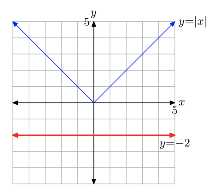
|x| = −2
- Answer
-
No solutions.
|x| = 0
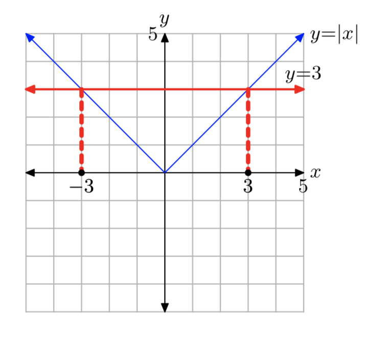
|x| = 3
- Answer
-
Solution: x = −3 or x = 3.
|x| = 2
For each of the equations in Exercises 5-8, perform each of the following tasks.
- Load each side of the equation into the Y= menu of your calculator. Ad- just the viewing window so that all points of intersection of the two graphs are visible in the viewing window.
- Copy the image in your viewing screen onto your homework paper. Label each axis and scale each axis with xmin, xmax, ymin, and ymax. Label each graph with its equation.
- Use the intersect utility in the CALC menu to determine the points of intersection. Shade and label each solution as shown in Figure 5 (read "Expectations") in the narrative. That is, drop dashed lines from the points of intersection to the axis, then shade and label the solution set on the x-axis.
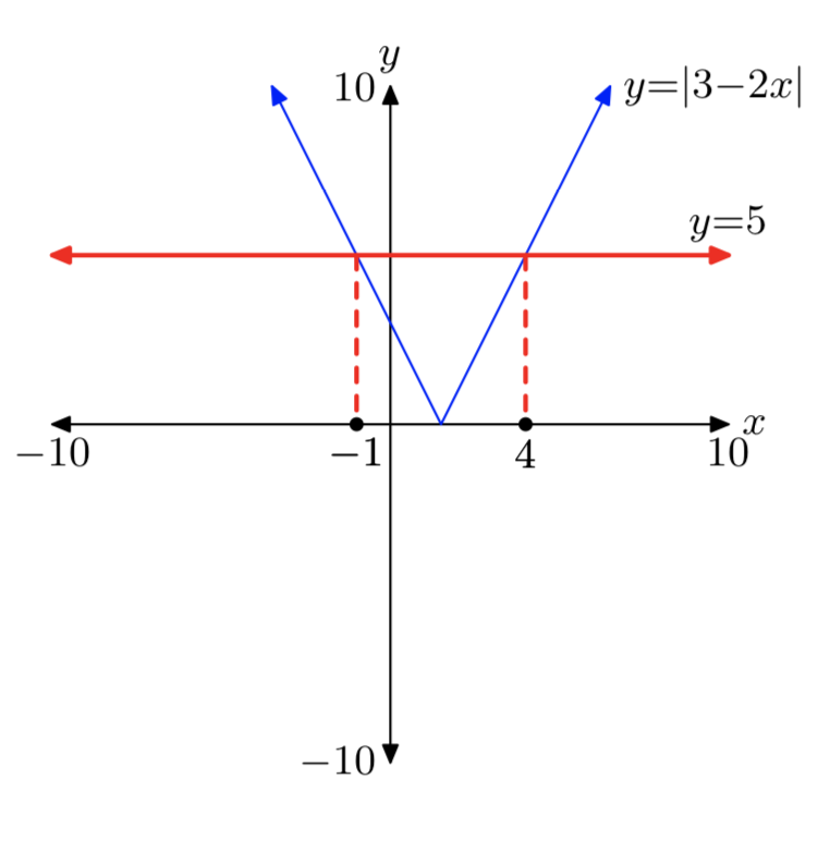
|3−2x| = 5
- Answer
-
Solutions: x = −1 or x = 4.
|2x+7| = 4
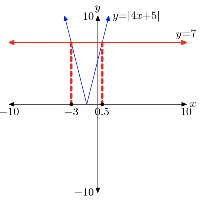
|4x+5| = 7
- Answer
-
Solutions: x = −3 or x = 0.5.
|5x−7| = 8
For each of the equations in Exercises 9-14, provide a purely algebraic solution without the use of a calculator. Arrange your work as shown in Examples 6, 7, and 8 in the narrative, but do not use a calculator.
|4x+3| = 0
- Answer
-
\(x = −\frac{3}{4}\)
|3x−11| = −5
|2x+7| = 14
- Answer
-
\(x = −\frac{21}{2}\) or \(x = \frac{7}{2}\)
|7−4x| = 8
|3−2x| = −1
- Answer
-
No solutions.
|4x+9| = 0
For each of the equations in Exercises 15-20, perform each of the following tasks.
- Arrange each of the following parts on your homework paper in the same location. Do not do place the algebraic work on one page and the graphical work on another.
- Follow each of the directions given for Exercises 5-8 to find and record a solution with your graphing calculator.
- Provide a purely algebraic solution, showing all the steps of your work. Do these solutions compare favorably with those found using your graphing calculator in part (ii)? If not, look for a mistake in your work.
|x−8| = 7
- Answer
-
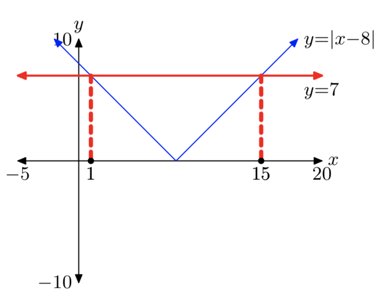
x = 1 or x = 15
|2x−15| = 5
|2x+11| = 6
- Answer
-
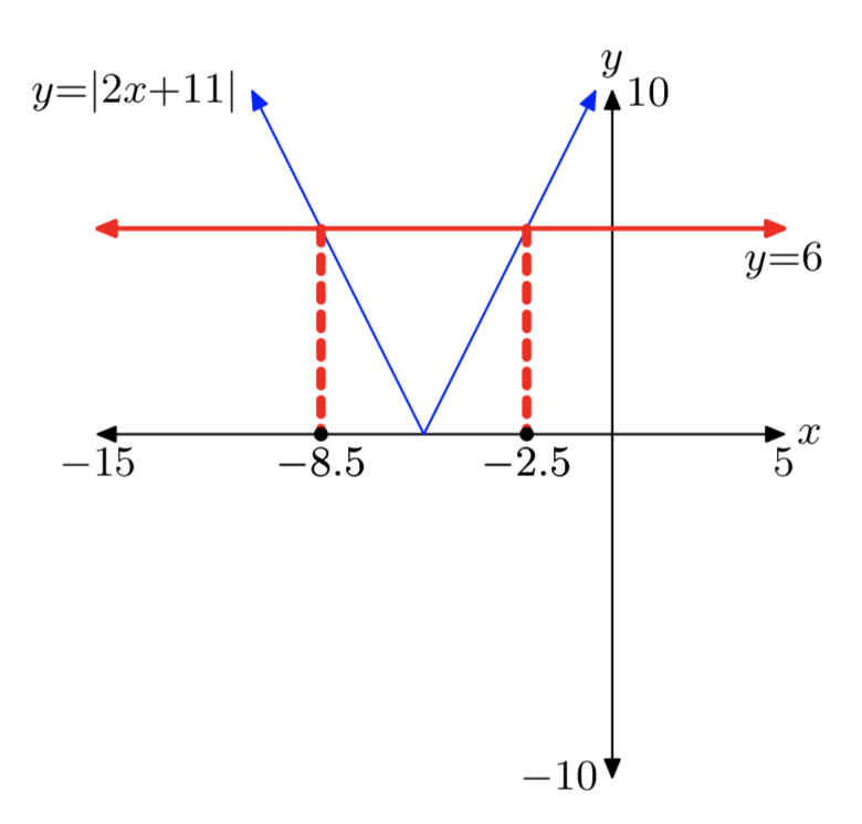
x = −8.5 or x = −2.5
|5x−21| = 7
|x−12| = 6
- Answer
-
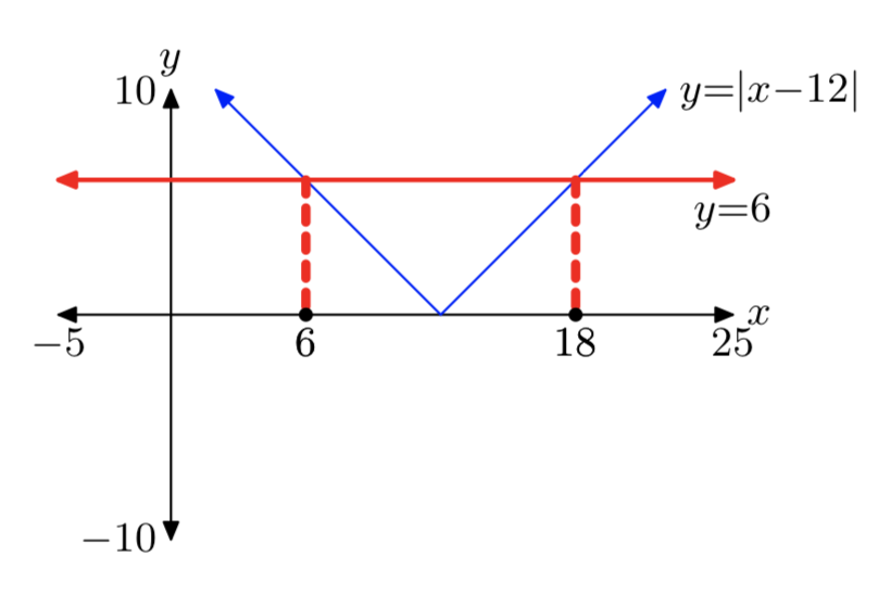
x = 6 or x = 18
|x+11| = 5
Use a strictly algebraic technique to solve each of the equations in Exercises 21-28. Do not use a calculator.
|x+2|−3 = 4
- Answer
-
x = −9 or x = 5
3|x+5| = 6
−2|3−2x| = −6
- Answer
-
x = 0 or x = 3
|4−x|+5 = 12
3|x+2|−5 = |x+2|+7
- Answer
-
x = −8 or x = 4
4−3|4−x| = 2|4−x|−1
\(|\frac{x}{3}−\frac{1}{4}| = \frac{1}{12}\)
- Answer
-
\(x = \frac{1}{2}\) or x = 1
\(|\frac{x}{4}−\frac{1}{2}| = \frac{2}{3}\)
Use the technique of distance on the number line demonstrated in Examples 16 and 17 to solve each of the equations in Exercises 29-32. Provide number line sketches on your homework paper as shown in Examples 16 and 17 in the narrative.
|x−5| = 8
- Answer
-

x = −3 or x = 13
|x−2| = 4
|x+4| = 3
- Answer
-

x = −7 or x = −1
|x+2| = 11
Use the instructions provided in Exercises 5-8 to solve the equations in Exercises 33-34.
\(|x+2| = \frac{1}{3}x+5\)
- Answer
-
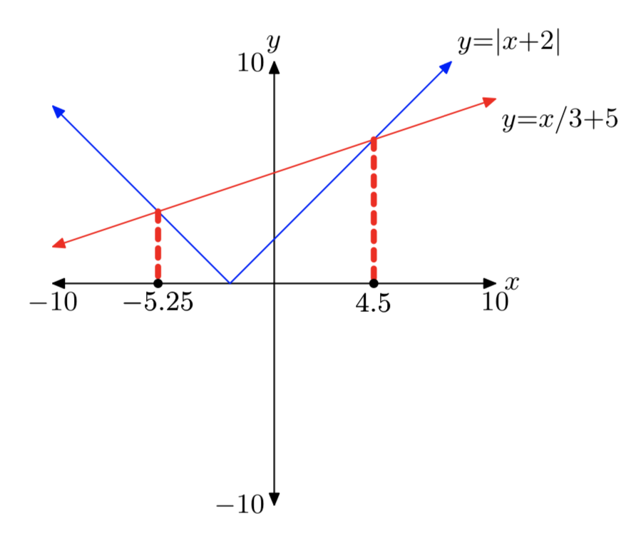
\(|x−3|=5−\frac{1}{2}x\)
In Exercises 35-36, perform each of the following tasks.
- Set up a coordinate system on graph paper. Label and scale each axis.
- Without the use of a calculator, sketch the graphs of the left- and right-hand sides of the given equation. Label each graph with its equation.
- Drop dashed vertical lines from each point of intersection to the x-axis. Shade and label each solution on the x-axis (you will have to approximate).
\(|x−2| = \frac{1}{3}x+2\)
- Answer
-
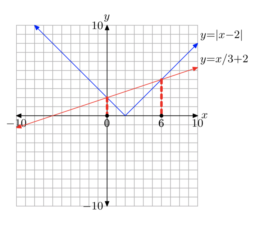
\(|x+4| = \frac{1}{3}x+4\)
Given that a < 0 and b > 0, prove that |ab| = |a||b|.
- Answer
-
If a is a negative real number and b is a positive real number, then ab is negative, so |ab| = −ab. On the other hand, a negative also means that |a| = −a, and b positive means that |b| = b, so that |a||b| = −a(b) = −ab. Comparing these results, we see that |ab| and |a||b| equal the same thing, and so they must be equal to one another.
Given that a>0 and b<0, prove that |ab| = |a||b|.
In the narrative, we proved that if a > 0 and b < 0, then \(|\frac{a}{b}| = \frac{|a|}{|b|}\). Prove the remaining three cases.
- Answer
-
CaseI. (a, b > 0) If a and b are both positive real numbers, then \(\frac{a}{b}\) is positive and so \(|\frac{a}{b}| = \frac{a}{b}\). On the other hand, a positive also means that |a| = a, and b positive means that |b| = b, so that \(\frac{|a|}{|b|} = \frac{a}{b}\). Comparing these two results, we see that \(|\frac{a}{b}|\) and \(\frac{|a|}{|b|}\) equal the same thing, and so they must be equal to one another.
Case II. (a, b < 0) If a and b are both negative real numbers, then \(\frac{a}{b}\) is positive and so \(|\frac{a}{b}| = \frac{a}{b}\). On the other hand, a negative also means that |a| = −a, and b negative means that |b| = −b, so that \(\frac{|a|}{|b|} = \frac{−a}{(−b)} = \frac{a}{b}\). Comparing these two results, we see that \(|\frac{a}{b}|\) and \(\frac{|a|}{|b|}\) equal the same thing, and so they must be equal to one another.
Case III. (a < 0, b > 0) If a is a negative real number and b is a positive real number, then \(\frac{a}{b}\) is negative and so \(|\frac{a}{b}| =−(\frac{a}{b})\). On the other hand, a negative also means that |a| = −a, and b positive means that |b| = b, so that \(\frac{|a|}{|b|} = −\frac{a}{b} = −(\frac{a}{b})\). Comparing these two results, we see that \(|\frac{a}{b}|\) and \(\frac{|a|}{|b|}\) equal the same thing, and so they must be equal to one another.


