10.2: Goodness-of-Fit Test

40

Goodness-of-Fit Test

jkesler

[latexpage]

In this type of hypothesis test, you determine whether the data “fit” a particular distribution or not. For example, you may suspect your unknown data fit a binomial distribution. You use a chi-square test (meaning the distribution for the hypothesis test is chi-square) to determine if there is a fit or not. The null and the alternative hypotheses for this test may be written in sentences or may be stated as equations or inequalities.

The test statistic for a goodness-of-fit test is:

$$\sum_k \frac{(O-E)^2}{E}$$

where:

• O = observed values (data)
• E = expected values (from theory)
• k = the number of different data cells or categories

The observed values are the data values and the expected values are the values you would expect to get if the null hypothesis were true. There are k terms of the form $\frac{(O-E)^2}{E}$.

The number of degrees of freedom is df = (number of categories – 1) = k – 1

The goodness-of-fit test is almost always right-tailed. If the observed values and the corresponding expected values are not close to each other, then the test statistic can get very large and will be way out in the right tail of the chi-square curve.

Note

The expected value for each cell needs to be at least five in order for you to use this test.

Example 10.1

Absenteeism of college students from math classes is a major concern to math instructors because missing class appears to increase the drop rate. Suppose that a study was done to determine if the actual student absenteeism rate follows faculty perception. The faculty expected that a group of 100 students would miss class according to Table 10.1.

Number of absences per term	Expected number of students
0–2	50
3–5	30
6–8	12
9–11	6
12+	2

Table 10.1

A random survey across all mathematics courses was then done to determine the actual number (observed) of absences in a course. The chart in Table 10.2 displays the results of that survey.

Number of absences per term	Actual number of students
0–2	35
3–5	40
6–8	20
9–11	1
12+	4

Table 10.2

Determine the null and alternative hypotheses needed to conduct a goodness-of-fit test.

H₀: Student absenteeism fits faculty perception.

The alternative hypothesis is the opposite of the null hypothesis.

H₁: Student absenteeism does not fit faculty perception.

a. Can you use the information as it appears in the charts to conduct the goodness-of-fit test?

Solution 10.1

a. No. Notice that the expected number of absences for the “12+” entry is less than five (it is two). Combine that group with the “9–11” group to create new tables where the number of students for each entry are at least five. The new results are in Table 10.3 and Table 10.4.

Number of absences per term	Expected number of students
0–2	50
3–5	30
6–8	12
9+	8

Table 10.3

Number of absences per term	Actual number of students
0–2	35
3–5	40
6–8	20
9+	5

Table 10.4

b. What is the number of degrees of freedom (df)?

Solution 10.1

b. There are four “cells” or categories in each of the new tables.

df = number of cells – 1 = 4 – 1 = 3

Try It 10.1

A factory manager needs to understand how many products are defective versus how many are produced. The number of expected defects is listed in Table 10.5.

Number produced	Number defective
0–100	5
101–200	6
201–300	7
301–400	8
401–500	10

Table 10.5

A random sample was taken to determine the actual number of defects. Table 10.6 shows the results of the survey.

Number produced	Number defective
0–100	5
101–200	7
201–300	8
301–400	9
401–500	11

Table 10.6

State the null and alternative hypotheses needed to conduct a goodness-of-fit test, and state the degrees of freedom.

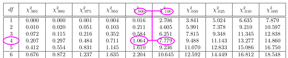
In the following Example 10.2, our solution will use the p-value method where we find the p-value corresponding to our test statistic and compare it with the significance level given.

In Example 10.3, our solution will use the critical value method where we find the critical value corresponding to the given significance level, and compare the critical value to the test statistic.

The p-value method and the critical value method are equivalent when determining whether to reject or fail to reject the null hypothesis.

Example 10.2

Employers want to know which days of the week employees are absent in a five-day work week. Most employers would like to believe that employees are absent equally during the week. Suppose a random sample of 60 managers were asked on which day of the week they had the highest number of employee absences. The results were distributed as in Table 10.7. For the population of employees, do the days for the highest number of absences occur with equal frequencies during a five-day work week? Test at a 5% significance level.

	Monday	Tuesday	Wednesday	Thursday	Friday
Number of Absences	15	12	9	9	15

Table 10.7Day of the Week Employees were Most Absent

Solution 10.2

The null and alternative hypotheses are:

• H₀: The absent days occur with equal frequencies, that is, they fit a uniform distribution.
• H₁: The absent days occur with unequal frequencies, that is, they do not fit a uniform distribution.

If the absent days occur with equal frequencies, then, out of 60 absent days (the total in the sample: 15 + 12 + 9 + 9 + 15 = 60), there would be 12 absences on Monday, 12 on Tuesday, 12 on Wednesday, 12 on Thursday, and 12 on Friday. These numbers are the expected (E) values. The values in the table are the observed (O) values or data.

This time, calculate the χ² test statistic by hand. Make a chart with the following headings and fill in the columns:

• Expected (E) values (12, 12, 12, 12, 12)
• Observed (O) values (15, 12, 9, 9, 15)
• (O – E)
• (O – E)²
• $\frac{(O-E)^2}{E}$

Day of Absences	$O$	$E$	$O – E$	$(O – E)^2$	$\frac{(O – E)^2}{E}$
Monday	15	12	3	9	0.75
Tuesday	12	12	0	0	0
Wednesday	9	12	-3	9	0.75
Thursday	9	12	-3	9	0.75
Friday	15	12	3	9	0.75

Now add the last column. $\sum \frac{(O-E)^2}{E} = 3$.

To find the p-value, calculate P(χ² > 3). First notice that df = k – 1 = 5 – 1 = 4. This test is right-tailed. You can use the Google Sheets formula
=CHISQ.DIST.RT(3,4)
to find p-value is approximately 0.5578

The dfs are the number of cells – 1 = 5 – 1 = 4

Figure 10.4

The decision is not to reject the null hypothesis.

Conclusion: At a 5% level of significance, from the sample data, there is not sufficient evidence to conclude that the absent days do not occur with equal frequencies.

You can use a Chi-square distribution table to find the range that contains the correct p-value. Usually, this is enough to draw a conclusion about a hypothesis test.

p-value Method

In this example, once you’ve calculated the test statistic, look in row 4 (since our df = 4). In this row, find the two numbers that are above and below our test statistic 3. Then follow those columns up to find which two values are above and below our p-value.

Chi2Distribution

The range of the p-value is 0.1 < p-value < 0.9 which tells us that it is larger than the significance level 0.05, so we fail to reject the null hypothesis (as we determined using Google Sheets as well).

Critical Value Method

Alternatively, we could get the critical value and compare it to the test statistic.

Find the column with the significance level 0.05 in the top row, then go down to row 4 (df = 4) and that is your critical value.

Our test statistic $\chi^2 = 3$ is not larger than the critical value 9.488, so we fail to reject the null hypothesis.

 

Try It 10.2

Teachers want to know which night each week their students are doing most of their homework. Most teachers think that students do homework equally throughout the week. Suppose a random sample of 56 students were asked on which night of the week they did the most homework. The results were distributed as in Table 10.8.

	Sunday	Monday	Tuesday	Wednesday	Thursday	Friday	Saturday
Number of Students	11	8	10	7	10	5	5

Table 10.8

From the population of students, do the nights for the highest number of students doing the majority of their homework occur with equal frequencies during a week? What type of hypothesis test should you use?

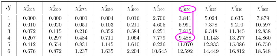
Example 10.3

One study indicates that the number of televisions that American families have is distributed (this is the given distribution for the American population) as in Table 10.9.

Number of Televisions	Percent
0	10
1	16
2	55
3	11
4+	8

Table 10.9

The table contains expected (E) percents.

A random sample of 600 families in the far western United States resulted in the data in Table 10.10.

Number of Televisions	Frequency
	Total = 600
0	66
1	119
2	340
3	60
4+	15

Table 10.10

The table contains observed (O) frequency values.

At the 1% significance level, does it appear that the distribution “number of televisions” of far western United States families is different from the distribution for the American population as a whole?

Solution 10.3

This problem asks you to test whether the far western United States families distribution fits the distribution of the American families. This test is always right-tailed.

The first table contains expected percentages. To get expected (E) frequencies, multiply the percentage by 600. The expected frequencies are shown in Table 10.11.

Number of Televisions	Percent	Expected Frequency
0	10	(0.10)(600) = 60
1	16	(0.16)(600) = 96
2	55	(0.55)(600) = 330
3	11	(0.11)(600) = 66
over 3	8	(0.08)(600) = 48

Table 10.11

Therefore, the expected frequencies are 60, 96, 330, 66, and 48.

H₀: The “number of televisions” distribution of far western United States families is the same as the “number of televisions” distribution of the American population.

H₁: The “number of televisions” distribution of far western United States families is different from the “number of televisions” distribution of the American population.

Distribution for the test: “>χ24

$\chi_4^2$ where df = (the number of cells) – 1 = 5 – 1 = 4.

Note

df ≠ 600 – 1

Calculate the test statistic:

Number of Televisions	$O$	$E$	$O – E$	$(O – E)^2$	$\frac{(O – E)^2}{E}$
0	66	60	6	36	0.6
1	119	96	23	529	5.510
2	340	330	10	100	0.303
3	60	66	-6	36	0.545
over 3	15	48	-33	1089	22.688

Now add the last column. $\sum \frac{(O-E)^2}{E} = 29.65$.

Find the critical value: Either use the Chi-square distribution table as described in the note at the bottom of Example 10.2 or use the following Google Sheets function noting the given significance level is 0.01 and the degrees of freedom df = k – 1 = 5 – 1 = 4:

=CHISQ.INV.RT(0.01,4)

We get a critical value 13.276

Compare the test statistic and critical value:

• test statistic $\chi^2 = 29.65$
  
• critical value is 13.276
  

So, the test statistic is further into the right tail than the critical value.

Make a decision: Since the test statistic is larger than (further to the right) the critical value, reject H_o.

This means you reject the belief that the distribution for the far western states is the same as that of the American population as a whole.

Conclusion: At the 1% significance level, from the data, there is sufficient evidence to conclude that the “number of televisions” distribution for the far western United States is different from the “number of televisions” distribution for the American population as a whole.

Try It 10.3

The expected percentage of the number of pets students have in their homes is distributed (this is the given distribution for the student population of the United States) as in Table 10.12.

Number of Pets	Percent
0	18
1	25
2	30
3	18
4+	9

Table 10.12

A random sample of 1,000 students from the Eastern United States resulted in the data in Table 10.13.

Number of Pets	Frequency
0	210
1	240
2	320
3	140
4+	90

Table 10.13

At the 1% significance level, does it appear that the distribution “number of pets” of students in the Eastern United States is different from the distribution for the United States student population as a whole? What is the p-value?

Example 10.4

Suppose you flip two coins 100 times. The results are 20 HH, 27 HT, 30 TH, and 23 TT. Are the coins fair? Test at a 5% significance level.

Solution 10.4

This problem can be set up as a goodness-of-fit problem. The sample space for flipping two fair coins is {HH, HT, TH, TT}. Out of 100 flips, you would expect 25 HH, 25 HT, 25 TH, and 25 TT. This is the expected distribution. The question, “Are the coins fair?” is the same as saying, “Does the distribution of the coins (20 HH, 27 HT, 30 TH, 23 TT) fit the expected distribution?”

Random Variable: Let X = the number of heads in one flip of the two coins. X takes on the values 0, 1, 2. (There are 0, 1, or 2 heads in the flip of two coins.) Therefore, the number of cells is three. Since X = the number of heads, the observed frequencies are 20 (for two heads), 57 (for one head), and 23 (for zero heads or both tails). The expected frequencies are 25 (for two heads), 50 (for one head), and 25 (for zero heads or both tails). This test is right-tailed.

H₀: The coins are fair.

H₁: The coins are not fair.

Distribution for the test:

$\chi_2^2$ where df = 3 – 1 = 2.

Calculate the test statistic:

	$O$	$E$	$O – E$	$(O – E)^2$	$\frac{(O – E)^2}{E}$
HH	20	25	-5	25	1
HT	27	25	2	4	0.16
TH	30	25	5	25	1
TT	23	25	-2	4	0.16

χ² = 2.32

Probability statement:p-value = P(χ² > 2.32) = 0.5087 using the Google Sheets function
=CHISQ.DIST.RT(2.32,3)

Compare α and the p-value:

• α = 0.05
• p-value = 0.5087

α < p-value.

Make a decision: Since α < p-value, do not reject H₀.

Conclusion: There is insufficient evidence to conclude that the coins are not fair.

Try It 10.4

Students in a social studies class hypothesize that the literacy rates across the world for every region are 82%. Table 10.14 shows the actual literacy rates across the world broken down by region. What are the test statistic and the degrees of freedom?

MDG Region	Adult Literacy Rate (%)
Developed Regions	99.0
Commonwealth of Independent States	99.5
Northern Africa	67.3
Sub-Saharan Africa	62.5
Latin America and the Caribbean	91.0
Eastern Asia	93.8
Southern Asia	61.9
South-Eastern Asia	91.9
Western Asia	84.5
Oceania	66.4

Table 10.14