9.3: Matched or Paired Samples

38

Matched or Paired Samples

jkesler

[latexpage]

When using a hypothesis test for matched or paired samples, the following characteristics should be present:

1. Simple random sampling is used.
2. Sample sizes are often small.
3. Two measurements (samples) are drawn from the same pair of individuals or objects.
4. Differences are calculated from the matched or paired samples.
5. The differences form the sample that is used for the hypothesis test.
6. Either the matched pairs have differences that come from a population that is normal or the number of differences is sufficiently large so that distribution of the sample mean of differences is approximately normal.

In a hypothesis test for matched or paired samples, subjects are matched in pairs and differences are calculated. The differences are the data. The population mean for the differences, μ_d, is then tested using a Student’s-t test for a single population mean with n – 1 degrees of freedom, where n is the number of differences.

We use $\bar x_d$ to represent the mean of the differences in our sample, and $s_d$ is the standard deviation of the differences in our sample. If you didn’t guess it, the subscript “d” stands for “differences”.

 

The test statistic (t-score) is:

$$t=\frac{\bar x_d-\mu_d}{\frac{s_d}{\sqrt{n}}}$$

The null hypothesis for these situations will always be
H₀: μ_d = 0 so we can write a simplified version of the test statistic as
$$t=\frac{\bar x_d}{\frac{s_d}{\sqrt{n}}}$$

 

Example 9.11

A study was conducted to investigate the effectiveness of hypnotism in reducing pain. Results for randomly selected subjects are shown in Table 9.11. A lower score indicates less pain. The “before” value is matched to an “after” value and the differences are calculated. The differences have a normal distribution. Are the sensory measurements, on average, lower after hypnotism? Test at a 5% significance level.

Subject:	A	B	C	D	E	F	G	H
Before	6.6	6.5	9.0	10.3	11.3	8.1	6.3	11.6
After	6.8	2.4	7.4	8.5	8.1	6.1	3.4	2.0

Table 9.11

Solution 9.11

Corresponding “before” and “after” values form matched pairs. (Calculate “after” – “before.”)

If you copy and paste the data into Google Sheets, you can easily calculate the differences into a third column. See the not on copying data that is given in rows into columns.

Before Data	After Data	Difference
6.6	6.8	-0.2
6.5	2.4	4.1
9	7.4	1.6
10.3	8.5	1.8
11.3	8.1	3.2
8.1	6.1	2
6.3	3.4	2.9
11.6	2	9.6

Table 9.12

The data for the test are the differences: {-0.2, 4.1, 1.6, 1.8, 3.2, 2, 2.9, 9.6}

The sample mean and sample standard deviation of the differences are:

$\bar x_d = 3.13$ and $s_d=2.91$

Verify these values by copying and pasting the data into Google Sheets and using the AVERAGE and STDEV.S functions on the column of differences.

Random variable:
“>X¯¯¯d

$\bar X_2$ is the mean difference of the sensory measurements

H₀: μ_d = 0

The null hypothesis is zero or positive, meaning that there is the same or more pain felt after hypnotism. That means the subject shows no improvement. μ_d is the population mean of the differences.)

H₁: μ_d >0

The alternative hypothesis is positive, meaning there is less pain felt after hypnotism. That means the subject shows improvement. The score should be lower after hypnotism, so the difference ought to be positive to indicate improvement.

Distribution for the test: The distribution is a Student’s t with df = n – 1 = 8 – 1 = 7. Use t₇. (Notice that the test is for a single population mean.)

Calculate the test statistic:

$t=\frac{\bar x_d}{\frac{s_d}{\sqrt{n}}}=\frac{ 3.13}{\frac{2.91}{\sqrt{8}}}=3.042$

Calculate the p-value using the Student’s t-distribution:p-value = 0.0094 using Google sheets
=TDIST(3.042,7,1)
We always use the positive version of the test statistic (even if it was negative) for the first value since the TDIST function only allows positive values. The second value is the degrees of freedom. The third value is the number of tails.

Compare α and the p-value:α = 0.05 and p-value = 0.0095. α > p-value.

Make a decision: Since α > p-value, reject H₀. This means that μ_d < 0 and there is improvement.

Conclusion: At a 5% level of significance, from the sample data, there is sufficient evidence to conclude that the sensory measurements, on average, are lower after hypnotism. Hypnotism appears to be effective in reducing pain.

Transposing Data in Google Sheets

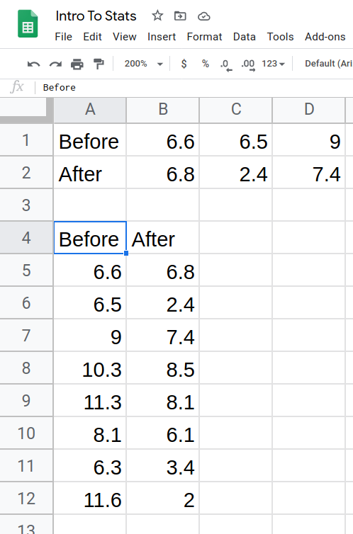
In this example, data was given to us in rows, but often we like to work with it in columns. This is called “transposing” the data in a spreadsheet. To do this in Google Sheets, follow these steps.

1. Copy the data from the problem into a Google Sheet. Then, select all the data copy using Ctrl-C or Command-C
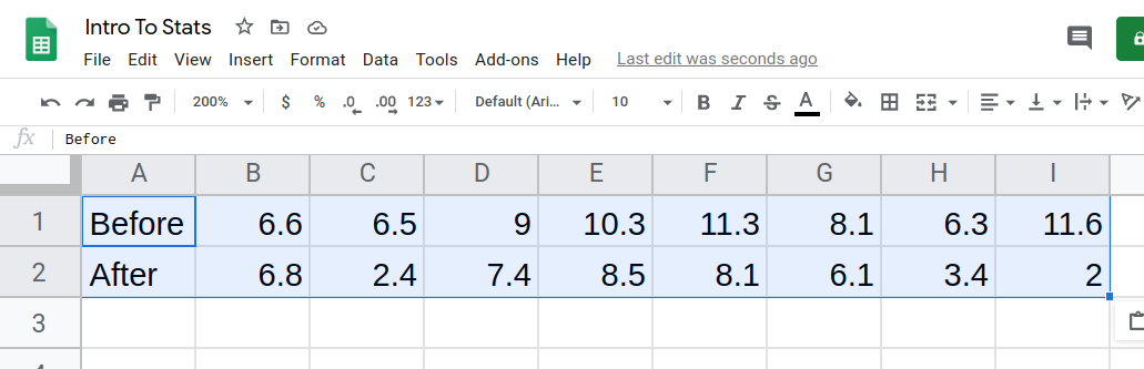
2. Choose a blank cell by clicking into it. In the top menu, click Edit, hover over Paste special, and click Paste transposed.
   
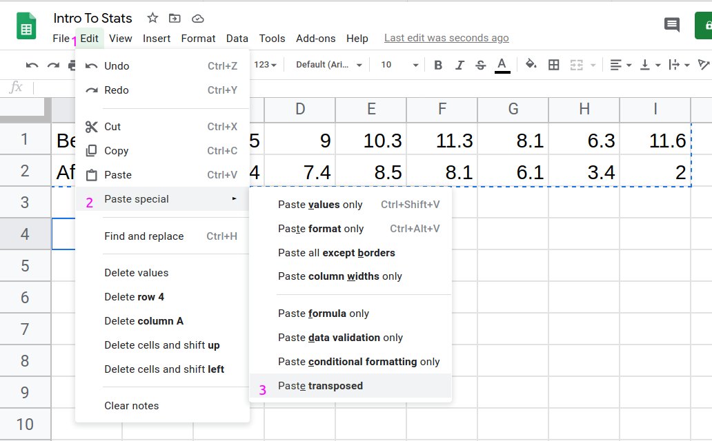
3. The data should now be presented in columns.
   

Try It 9.11

A study was conducted to investigate how effective a new diet was in lowering cholesterol. Results for the randomly selected subjects are shown in the table. The differences have a normal distribution. Are the subjects’ cholesterol levels lower on average after the diet? Test at the 5% level.

Subject	A	B	C	D	E	F	G	H	I
Before	209	210	205	198	216	217	238	240	222
After	199	207	189	209	217	202	211	223	201

Table 9.13

Example 9.12

A college football coach was interested in whether the college’s strength development class increased his players’ maximum lift (in pounds) on the bench press exercise. He asked four of his players to participate in a study. The amount of weight they could each lift was recorded before they took the strength development class. After completing the class, the amount of weight they could each lift was again measured. The data are as follows:

Weight (in pounds)	Player 1	Player 2	Player 3	Player 4
Amount of weight lifted prior to the class	205	241	338	368
Amount of weight lifted after the class	295	252	330	360

Table 9.14

The coach wants to know if the strength development class makes his players stronger, on average.

Record the differences data. Calculate the differences by subtracting the amount of weight lifted prior to the class from the weight lifted after completing the class. The data for the differences are: {90, 11, -8, -8}. Assume the differences have a normal distribution.

Using the differences data, calculate the sample mean and the sample standard deviation

$\bar x_d = 21.3$ and $s_d = 46.7$

Note

The data given here would indicate that the distribution is actually right-skewed. The difference 90 may be an extreme outlier? It is pulling the sample mean to be 21.3 (positive). The means of the other three data values are actually negative.

Using the difference data, this becomes a test of a single __________ (fill in the blank).

Define the random variable: “>X¯¯¯d

$\bar X_d$ mean difference in the maximum lift per player.

The distribution for the hypothesis test is t₃.

H₀: μ_d = 0, H₁: μ_d > 0

Calculate the test statistic:

$t=\frac{\bar x_d}{\frac{s_d}{\sqrt{n}}}=\frac{ 21.3}{\frac{46.7}{\sqrt{4}}}=0.912$

Calculate the p-value:

The p-value is 0.2145 using Google Sheets
=tdist(0.912,3,1)

Decision: If the level of significance is 5%, the decision is not to reject the null hypothesis, because α < p-value.

What is the conclusion?

At a 5% level of significance, from the sample data, there is not sufficient evidence to conclude that the strength development class helped to make the players stronger, on average.

Try It 9.12

A new prep class was designed to improve SAT test scores. Five students were selected at random. Their scores on two practice exams were recorded, one before the class and one after. The data recorded in Table 9.15. Are the scores, on average, higher after the class? Test at a 5% level.

SAT Scores	Student 1	Student 2	Student 3	Student 4
Score before class	1840	1960	1920	2150
Score after class	1920	2160	2200	2100

Table 9.15

Example 9.13

Seven eighth graders at Kennedy Middle School measured how far they could push the shot-put with their dominant (writing) hand and their weaker (non-writing) hand. They thought that they could push equal distances with either hand. The data were collected and recorded in Table 9.16.

Distance (in feet) using	Student 1	Student 2	Student 3	Student 4	Student 5	Student 6	Student 7
Dominant Hand	30	26	34	17	19	26	20
Weaker Hand	28	14	27	18	17	26	16

Table 9.16

Solution 9.13

Conduct a hypothesis test to determine whether the mean difference in distances between the children’s dominant versus weaker hands is significant.

Record the differences data. Calculate the differences by subtracting the distances with the weaker hand from the distances with the dominant hand. The data for the differences are: {2, 12, 7, –1, 2, 0, 4}. The differences have a normal distribution.

Using the differences data, calculate the sample mean and the sample standard deviation. “>x¯d

$\bar x_d= 3.71$, and $s_d = 4.5$

Random variable: “>X¯¯¯d

$\bar X_d$ = mean difference in the distances between the hands.

Distribution for the hypothesis test:t₆

H₀: μ_d = 0 H₁: μ_d ≠ 0

Calculate the test statistic:

$t=\frac{\bar x_d}{\frac{s_d}{\sqrt{n}}}=\frac{ 3.71}{\frac{4.5}{\sqrt{7}}}=2.181$

Calculate the p-value:
The p-value is 0.072 using Google Sheets
=TDIST(2.181,6,2)

The last value given to the TDIST function is a 2 since this is a two-tail test.

Decision: Assume α = 0.05. Since α < p-value, Do not reject H₀.

Conclusion: At the 5% level of significance, from the sample data, there is not sufficient evidence to conclude that there is a difference in the children’s weaker and dominant hands to push the shot-put.

Try It 9.13

Five ball players think they can throw the same distance with their dominant hand (throwing) and off-hand (catching hand). The data were collected and recorded in Table 9.17. Conduct a hypothesis test to determine whether the mean difference in distances between the dominant and off-hand is significant. Test at the 5% level.

	Player 1	Player 2	Player 3	Player 4	Player 5
Dominant Hand	120	111	135	140	125
Off-hand	105	109	98	111	99

Table 9.17