6.2: Central Limit Theorem for Sums

26

Central Limit Theorem for Sums

jkesler

[latexpage]

Suppose X is a random variable with a distribution that may be known or unknown (it can be any distribution) and suppose:

1. μ_X = the mean of Χ
2. σ_Χ = the standard deviation of X

If you draw random samples of size n, then as n increases, the random variable ΣX consisting of sums tends to be normally distributed and $\sum X \sim N \left( n\cdot \mu_x, \sqrt{n}\cdot \sigma_x \right)$

Thecentral limit theorem for sums says that if you repeatedly draw samples of a given size (such as repeatedly rolling ten dice) and calculate the sum of each sample, these sums tend to follow a normal distribution. As sample sizes increase, the distribution of means more closely follows the normal distribution. The normal distribution has a mean equal to the original mean multiplied by the sample size and a standard deviation equal to the original standard deviation multiplied by the square root of the sample size.

The random variable ΣX has the following z-score associated with it:

1. Σx is one sum.
2. $z = \frac{\sum x -n\cdot \mu_X}{\sqrt{n}\cdot \sigma_x}$
   1. $n\cdot \mu_x = $ the mean of $\sum X$
   2. $\sqrt{n}\cdot \sigma_X = $ the standard deviation of $\sum X$

Example 6.5

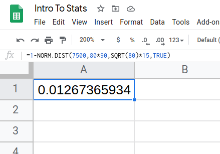
An unknown distribution has a mean of 90 and a standard deviation of 15. A sample of size 80 is drawn randomly from the population.

1. Find the probability that the sum of the 80 values (or the total of the 80 values) is more than 7,500.
2. Find the sum that is 1.5 standard deviations above the mean of the sums.

Solution 6.5

Let X = one value from the original unknown population. The probability question asks you to find a probability for the sum (or total of) 80 values.

ΣX = the sum or total of 80 values. Since μ_X = 90, σ_X = 15, and n = 80, $\sum X \sim N(80\cdot 90, \sqrt{80}\cdot 15)$ “>

• mean of the sums = $n\cdot \mu_X = 80\cdot 90 = 7,200$
• standard deviation of the sums = $\sqrt{80}\cdot 15)$ “>
• sum of 80 values = Σx = 7,500
  

1. Find P(Σx > 7,500)
   
   Figure 6.3

   Using Google Sheets
   

   =1-NORM.DIST(7500,80*90,SQRT(80)*15,TRUE)

   

   P(Σx > 7,500)= 0.0127

2. Find Σx where z = 1.5.$\sum x = n \cdot \mu_x + z \cdot \sqrt{n} \cdot \sigma_x = 80\cdot 90 + 1.5 \cdot \sqrt{80}\cdot 15 = 7,401.2$

Try It 6.5

An unknown distribution has a mean of 45 and a standard deviation of eight. A sample size of 50 is drawn randomly from the population. Find the probability that the sum of the 50 values is more than 2,400.

Using Google Sheets

To find percentiles for sums using a spreadsheet, use the NORM.INV function. Type the following in a cell:

=NORM.INV(k, n * mean, SQRT(n)*standard deviation)

where:

• k is the k^thpercentile
• mean is the mean of the original distribution
• standard deviation is the standard deviation of the original distribution
• sample size = n

Example 6.6

In a study reported Oct. 29, 2012 on the Flurry Blog, the mean age of tablet users is 34 years. Suppose the standard deviation is 15 years. The sample of size is 50.

1. What are the mean and standard deviation for the sum of the ages of tablet users? What is the distribution?
2. Find the probability that the sum of the ages is between 1,500 and 1,800 years.
3. Find the 80^th percentile for the sum of the 50 ages.

Solution 6.6

1. $\mu_{\sum x}=n\mu_{x}=1700$ and $\sigma_{\sum x}=\sqrt{n}~\sigma_{x} = \sqrt{50}\cdot 15 = 106.07$
   The distribution is normal for sums by the central limit theorem.
2. P(1500 < Σx < 1800) =
=NORM.DIST(1800,50*34, SQRT(50)*15,TRUE)-NORM.DIST(1500,50*34,SQRT(50)*15,TRUE)
   =0.7974
3. Let k = the 80^th percentile.
   k =
   =NORM.INV(0.80,50*34,SQRT(50)*15)
   =1,789.3

Try It 6.6

In a recent study reported Oct.29, 2012 on the Flurry Blog, the mean age of tablet users is 35 years. Suppose the standard deviation is ten years. The sample size is 39.

1. What are the mean and standard deviation for the sum of the ages of tablet users? What is the distribution?
2. Find the probability that the sum of the ages is between 1,400 and 1,500 years.
3. Find the 90^th percentile for the sum of the 39 ages.

Example 6.7

The mean number of minutes for app engagement by a tablet user is 8.2 minutes. Suppose the standard deviation is one minute. Take a sample of size 70.

1. What are the mean and standard deviation for the sums?
2. Find the 95^th percentile for the sum of the sample. Interpret this value in a complete sentence.
3. Find the probability that the sum of the sample is at least ten hours.

Solution 6.7

1. μ_Σx = nμ_x = 70(8.2) = 574 minutes and σ_Σx $=\sqrt{n}\cdot \sigma_x= \sqrt{70}\cdot 1 = 8.37$ minutes
2. Let k = the 95^th percentile.
   k =
   =NORM.INV(0.95, 70*8.2,SQRT(70)*1)
   = 587.76 minutes
   
   Ninety five percent of the sums of app engagement times are at most 587.76 minutes.
3. ten hours = 600 minutes
   
   P(Σx ≥ 600) =
   =1-NORM.DIST(600,70*8.2, SQRT(70)*1, TRUE)
   = 0.0009

Try It 6.7

The mean number of minutes for app engagement by a table use is 8.2 minutes. Suppose the standard deviation is one minute. Take a sample size of 70.

1. What is the probability that the sum of the sample is between seven hours and ten hours? What does this mean in context of the problem?
2. Find the 84^th and 16^th percentiles for the sum of the sample. Interpret these values in context.