4.2: Variability in Estimates

We would like to estimate two features of the Cherry Blossom runners using the sample.

1. How long does it take a runner, on average, to complete the 10 miles?
2. What is the average age of the runners?

These questions may be informative for planning the Cherry Blossom Run in future years.² We will use \(x_1, \dots, x_{100}\) to represent the 10 mile time for each runner in our sample, and \(y_1, \dots, y_{100}\) will represent the age of each of these participants.

²While we focus on the mean in this chapter, questions regarding variation are often just as important in practice. For instance, we would plan an event very differently if the standard deviation of runner age was 2 versus if it was 20.

Point Rstimates

We want to estimate the population mean based on the sample. The most intuitive way to go about doing this is to simply take the sample mean. That is, to estimate the average 10 mile run time of all participants, take the average time for the sample:

\[ \bar {x} = \frac {88.22 + 100.58 + \dots + 89.40}{100} = 95.61\]

The sample mean \(\bar {x}\) = 95.61 minutes is called a point estimate of the population mean: if we can only choose one value to estimate the population mean, this is our best guess. Suppose we take a new sample of 100 people and recompute the mean; we will probably not get the exact same answer that we got using the run10Samp data set. Estimates generally vary from one sample to another, and this sampling variation suggests our estimate may be close, but it will not be exactly equal to the parameter.

We can also estimate the average age of participants by examining the sample mean of age:

\[ \bar {y} = \frac {59 + 32 + \dots + 26}{100} = 35.05\]

What about generating point estimates of other population parameters, such as the population median or population standard deviation? Once again we might estimate parameters based on sample statistics, as shown in Table 4.5. For example, we estimate the population standard deviation for the running time using the sample standard deviation, 15.78 minutes.

Table 4.5: Point estimates and parameter values for the time variable.

time	estimate	parameter
mean median st. dev.	95.61 95.37 15.78	94.52 94.03 15.93

Exercise 4.1 Suppose we want to estimate the difference in run times for men and women. If \( \bar {x} _{men} = 87.65\) and \( \bar {x}_{women} = 102.13\), then what would be a good point estimate for the population difference?³

Exercise 4.2 If you had to provide a point estimate of the population IQR for the run time of participants, how might you make such an estimate using a sample?⁴

Point Estimates are not Exact

Estimates are usually not exactly equal to the truth, but they get better as more data become available. We can see this by plotting a running mean from our run10Samp sample. A running mean is a sequence of means, where each mean uses one more observation in its calculation than the mean directly before it in the sequence. For example, the second mean in the sequence is the average of the rst two observations and the third in the

³We could take the difference of the two sample means: 102.13 - 87.65 = 14.48. Men ran about 14.48 minutes faster on average in the 2012 Cherry Blossom Run.

⁴To obtain a point estimate of the IQR for the population, we could take the IQR of the sample.

Figure 4.6: The mean computed after adding each individual to the sample. The mean tends to approach the true population average as more data become available.

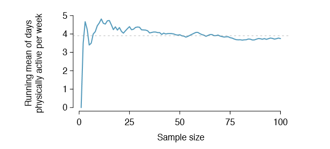
sequence is the average of the rst three. The running mean for the 10 mile run time in the run10Samp data set is shown in Figure 4.6, and it approaches the true population average, 94.52 minutes, as more data become available.

Sample point estimates only approximate the population parameter, and they vary from one sample to another. If we took another simple random sample of the Cherry Blossom runners, we would nd that the sample mean for the run time would be a little different. It will be useful to quantify how variable an estimate is from one sample to another. If this variability is small (i.e. the sample mean doesn't change much from one sample to another) then that estimate is probably very accurate. If it varies widely from one sample to another, then we should not expect our estimate to be very good.

Standard Error of the Mean

From the random sample represented in run10Samp, we guessed the average time it takes to run 10 miles is 95.61 minutes. Suppose we take another random sample of 100 individuals and take its mean: 95.30 minutes. Suppose we took another (93.43 minutes) and another (94.16 minutes), and so on. If we do this many many times { which we can do only because we have the entire population data set { we can build up a sampling distribution for the sample mean when the sample size is 100, shown in Figure 4.7.

Sampling distribution

The sampling distribution represents the distribution of the point estimates based on samples of a fixed size from a certain population. It is useful to think of a particular point estimate as being drawn from such a distribution. Understanding the concept of a sampling distribution is central to understanding statistical inference.

The sampling distribution shown in Figure 4.7 is unimodal and approximately symmetric. It is also centered exactly at the true population mean: \(\mu\) = 94.52. Intuitively, this makes sense. The sample means should tend to "fall around" the population mean.

We can see that the sample mean has some variability around the population mean, which can be quanti ed using the standard deviation of this distribution of sample means: \(\sigma _{\bar {x}} = 1.59\). The standard deviation of the sample mean tells us how far the typical estimate

Figure 4.7: A histogram of 1000 sample means for run time, where the samples are of size n = 100.

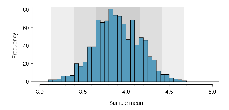
is away from the actual population mean, 94.52 minutes. It also describes the typical error of the point estimate, and for this reason we usually call this standard deviation the standard error (SE) of the estimate.

Standard error of an estimate

The standard deviation associated with an estimate is called the standard error. It describes the typical error or uncertainty associated with the estimate.

When considering the case of the point estimate \(\bar {x}\), there is one problem: there is no obvious way to estimate its standard error from a single sample. However, statistical theory provides a helpful tool to address this issue.

Exercise 4.3

1. Would you rather use a small sample or a large sample when estimating a parameter? Why?
2. Using your reasoning from (a), would you expect a point estimate based on a small sample to have smaller or larger standard error than a point estimate based on a larger sample?⁵

In the sample of 100 runners, the standard error of the sample mean is equal to onetenth of the population standard deviation: \(1.59 = \frac {15.93}{10}\). In other words, the standard error of the sample mean based on 100 observations is equal to

\[ SE_{\bar {x}} = \sigma_{\bar {x}} = \frac {\sigma_x}{\sqrt {100}} = \frac {15.93}{\sqrt {100}} = 1.59\]

where \(\sigma_x\) is the standard deviation of the individual observations. This is no coincidence. We can show mathematically that this equation is correct when the observations are independent using the probability tools of Section 2.4.

⁵(a) Consider two random samples: one of size 10 and one of size 1000. Individual observations in the small sample are highly inuential on the estimate while in larger samples these individual observations would more often average each other out. The larger sample would tend to provide a more accurate estimate. (b) If we think an estimate is better, we probably mean it typically has less error. Based on (a), our intuition suggests that a larger sample size corresponds to a smaller standard error.

Computing Standard Error for the sample mean

Given n independent observations from a population with standard deviation \(\sigma\), the standard error of the sample mean is equal to

\[ SE = \dfrac {\sigma}{\sqrt {n}} \tag {4.4}\]

A reliable method to ensure sample observations are independent is to conduct a simple random sample consisting of less than 10% of the population.

There is one subtle issue of Equation (4.4): the population standard deviation is typically unknown. You might have already guessed how to resolve this problem: we can use the point estimate of the standard deviation from the sample. This estimate tends to be sufficiently good when the sample size is at least 30 and the population distribution is not strongly skewed. Thus, we often just use the sample standard deviation s instead of \(\sigma\). When the sample size is smaller than 30, we will need to use a method to account for extra uncertainty in the standard error. If the skew condition is not met, a larger sample is needed to compensate for the extra skew. These topics are further discussed in Section 4.4.

Exercise 4.5 In the sample of 100 runners, the standard deviation of the runners' ages is \(s_y = 8.97\). Because the sample is simple random and consists of less than 10% of the population, the observations are independent. (a) What is the standard error of the sample mean, \(\bar {y} = 35.05\) years? (b) Would you be surprised if someone told you the average age of all the runners was actually 36 years?⁶

Exercise 4.6 (a)Would you be more trusting of a sample that has 100 observations or 400 observations? (b) We want to show mathematically that our estimate tends to be better when the sample size is larger. If the standard deviation of the individual observations is 10, what is our estimate of the standard error when the sample size is 100? What about when it is 400? (c) Explain how your answer to (b) mathematically justifies your intuition in part (a).⁷

Basic properties of point estimates

We achieved three goals in this section. First, we determined that point estimates from a sample may be used to estimate population parameters. We also determined that these point estimates are not exact: they vary from one sample to another. Lastly, we quantified the uncertainty of the sample mean using what we call the standard error, mathematically represented in Equation (4.4). While we could also quantify the standard error for other estimates - such as the median, standard deviation, or any other number of statistics - we will postpone these extensions until later chapters or courses.

⁶(a) Use Equation (4.4) with the sample standard deviation to compute the standard error: \(SE_{\bar {y}} = \frac {8.97}{\sqrt {100}} = 0.90\) years. (b) It would not be surprising. Our sample is about 1 standard error from 36 years. In other words, 36 years old does not seem to be implausible given that our sample was relatively close to it. (We use the standard error to identify what is close.)

⁷(a) Extra observations are usually helpful in understanding the population, so a point estimate with 400 observations seems more trustworthy. (b) The standard error when the sample size is 100 is given by \(SE_{100} = \frac {10}{\sqrt {100}} = 1\). For 400: \(SE_{400} = \frac {10}{\sqrt {400}} = 0.5\). The larger sample has a smaller standard error. (c) The standard error of the sample with 400 observations is lower than that of the sample with 100 observations. The standard error describes the typical error, and since it is lower for the larger sample, this mathematically shows the estimate from the larger sample tends to be better - though it does not guarantee that every large sample will provide a better estimate than a particular small sample.