4.3: Confidence Intervals

A point estimate provides a single plausible value for a parameter. However, a point estimate is rarely perfect; usually there is some error in the estimate. Instead of supplying just a point estimate of a parameter, a next logical step would be to provide a plausible range of values for the parameter.

In this section and in Section 4.3, we will emphasize the special case where the point estimate is a sample mean and the parameter is the population mean. In Section 4.5, we generalize these methods for a variety of point estimates and population parameters that we will encounter in Chapter 5 and beyond.

Capturing the population Parameter

A plausible range of values for the population parameter is called a confidence interval. Using only a point estimate is like fishing in a murky lake with a spear, and using a confidence interval is like shing with a net. We can throw a spear where we saw a fish, but we will probably miss. On the other hand, if we toss a net in that area, we have a good chance of catching the fish.

If we report a point estimate, we probably will not hit the exact population parameter. On the other hand, if we report a range of plausible values - a confidence interval - we have a good shot at capturing the parameter.

Exercise 4.7

If we want to be very certain we capture the population parameter, should we use a wider interval or a smaller interval?⁸

An Approximate 95% confidence interval

Our point estimate is the most plausible value of the parameter, so it makes sense to build the confidence interval around the point estimate. The standard error, which is a measure of the uncertainty associated with the point estimate, provides a guide for how large we should make the confidence interval.

The standard error represents the standard deviation associated with the estimate, and roughly 95% of the time the estimate will be within 2 standard errors of the parameter. If the interval spreads out 2 standard errors from the point estimate, we can be roughly 95% con dent that we have captured the true parameter:

\[ \text {point estimate} \pm 2 \times SE \label{4.8}\]

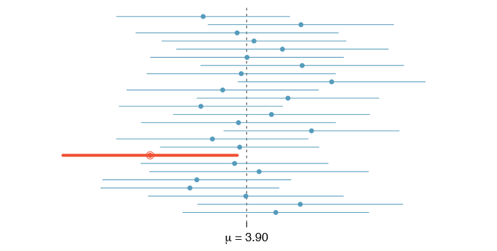
But what does "95% confident" mean? Suppose we took many samples and built a confidence interval from each sample using Equation \ref{4.8}. Then about 95% of those intervals would contain the actual mean, \(\mu\). Figure 4.8 shows this process with 25 samples, where 24 of the resulting confidence intervals contain the average time for all the runners, \(\mu = 94.52\) minutes, and one does not.

Exercise 4.9

In Figure 4.8, one interval does not contain 94.52 minutes. Does this imply that the mean cannot be 94.52? ⁹

Figure 4.8: Twenty- ve samples of size n = 100 were taken from the run10 data set. For each sample, a confidence interval was created to try to capture the average 10 mile time for the population. Only 1 of these 25 intervals did not capture the true mean, \(\mu = 94.52\) minutes.

⁸If we want to be more certain we will capture the sh, we might use a wider net. Likewise, we use a wider confidence interval if we want to be more certain that we capture the parameter.

⁹Just as some observations occur more than 2 standard deviations from the mean, some point estimates will be more than 2 standard errors from the parameter. A confidence interval only provides a plausible range of values for a parameter. While we might say other values are implausible based on the data, this does not mean they are impossible.

The rule where about 95% of observations are within 2 standard deviations of the mean is only approximately true. However, it holds very well for the normal distribution. As we will soon see, the mean tends to be normally distributed when the sample size is sufficiently large.

Example 4.10

If the sample mean of times from run10Samp is 95.61 minutes and the standard error, as estimated using the sample standard deviation, is 1.58 minutes, what would be an approximate 95% confidence interval for the average 10 mile time of all runners in the race? Apply the standard error calculated using the sample standard deviation (\(SE = \frac {15.78}{\sqrt {100}} = 1:58\)), which is how we usually proceed since the population standard deviation is generally unknown.

Solution

We apply Equation \ref{4.8}:

\[95.61 \pm 2 \times 1.58 \rightarrow (92.45, 98.77)\]

Based on these data, we are about 95% con dent that the average 10 mile time for all runners in the race was larger than 92.45 but less than 98.77 minutes. Our interval extends out 2 standard errors from the point estimate, \(\bar {x}\).

Exercise 4.11

he sample data suggest the average runner's age is about 35.05 years with a standard error of 0.90 years (estimated using the sample standard deviation, 8.97). What is an approximate 95% confidence interval for the average age of all of the runners?¹⁰

¹⁰Again apply Equation \ref{4.8}: \(35.05 \pm 2 \times 0.90 \rightarrow (33.25, 36.85)\). We interpret this interval as follows: We are about 95% con dent the average age of all participants in the 2012 Cherry Blossom Run was between 33.25 and 36.85 years.

A Sampling Distribution for the Mean

In Section 4.1.3, we introduced a sampling distribution for \(\bar {x}\), the average run time for samples of size 100. We examined this distribution earlier in Figure 4.7. Now we'll take 100,000 samples, calculate the mean of each, and plot them in a histogram to get an especially accurate depiction of the sampling distribution. This histogram is shown in the left panel of Figure 4.9.

Figure 4.9: The left panel shows a histogram of the sample means for 100,000 different random samples. The right panel shows a normal probability plot of those sample means.

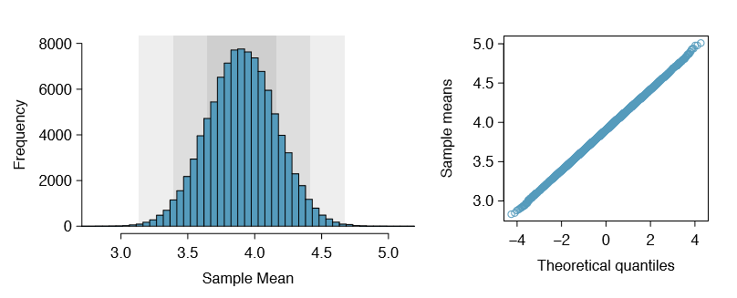
Does this distribution look familiar? Hopefully so! The distribution of sample means closely resembles the normal distribution (see Section 3.1). A normal probability plot of these sample means is shown in the right panel of Figure 4.9. Because all of the points closely fall around a straight line, we can conclude the distribution of sample means is nearly normal. This result can be explained by the Central Limit Theorem.

Central Limit Theorem, informal description

If a sample consists of at least 30 independent observations and the data are not strongly skewed, then the distribution of the sample mean is well approximated by a normal model.

We will apply this informal version of the Central Limit Theorem for now, and discuss its details further in Section 4.4.

The choice of using 2 standard errors in Equation\ref{4.8} was based on our general guideline that roughly 95% of the time, observations are within two standard deviations of the mean. Under the normal model, we can make this more accurate by using 1.96 in place of 2.

\[ \text {point estimate} \pm 1.96 \times SE \label{4.12}\]

If a point estimate, such as \( \bar {x}\), is associated with a normal model and standard error SE, then we use this more precise 95% confidence interval.

Changing the confidence level

Suppose we want to consider confidence intervals where the confidence level is somewhat higher than 95%: perhaps we would like a confidence level of 99%. Think back to the analogy about trying to catch a sh: if we want to be more sure that we will catch the fish, we should use a wider net. To create a 99% confidence level, we must also widen our 95% interval. On the other hand, if we want an interval with lower confidence, such as 90%, we could make our original 95% interval slightly slimmer.

The 95% confidence interval structure provides guidance in how to make intervals with new confidence levels. Below is a general 95% confidence interval for a point estimate that comes from a nearly normal distribution:

\[ \text {point estimate} \pm 1.96 \times SE \label{4.13}\]

There are three components to this interval: the point estimate, "1.96", and the standard error. The choice of 1:96 SE was based on capturing 95% of the data since the estimate is within 1.96 standard deviations of the parameter about 95% of the time. The choice of 1.96 corresponds to a 95% confidence level.

Exercise 4.14

If X is a normally distributed random variable, how often will X be within 2.58 standard deviations of the mean?¹¹

To create a 99% confidence interval, change 1.96 in the 95% confidence interval formula to be 2:58. Exercise 4.14 highlights that 99% of the time a normal random variable will be within 2.58 standard deviations of the mean. This approach - using the Z scores in the normal model to compute confidence levels - is appropriate when \( \bar {x}\) is associated with a normal distribution with mean \(\mu\) and standard deviation \(SE_{\bar {x}}\). Thus, the formula for a 99% confidence interval is

\[\bar {x} \pm 2.58 \times SE \bar {x} \label{4.15}\]

The normal approximation is crucial to the precision of these confidence intervals. Section 4.4 provides a more detailed discussion about when the normal model can safely be applied. When the normal model is not a good fit, we will use alternative distributions that better characterize the sampling distribution.

Conditions for \(\bar {x}\) being nearly normal and SE being accurate

Important conditions to help ensure the sampling distribution of \(\bar {x}\) is nearly normal and the estimate of SE sufficiently accurate:

• The sample observations are independent.
• The sample size is large: \(n \ge 30\) is a good rule of thumb.
• The distribution of sample observations is not strongly skewed.

Additionally, the larger the sample size, the more lenient we can be with the sample's skew.

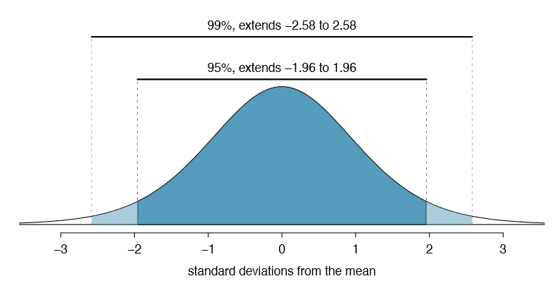
¹¹This is equivalent to asking how often the Z score will be larger than -2.58 but less than 2.58. (For a picture, see Figure 4.10.) To determine this probability, look up -2.58 and 2.58 in the normal probability table (0.0049 and 0.9951). Thus, there is a \(0.9951-0.0049 \approx 0.99\) probability that the unobserved random variable X will be within 2.58 standard deviations of \(\mu\).

Figure 4.10: The area between -z* and z* increases as |z*| becomes larger. If the confidence level is 99%, we choose z* such that 99% of the normal curve is between -z* and z*, which corresponds to 0.5% in the lower tail and 0.5% in the upper tail: z* = 2:58.

Verifying independence is often the most difficult of the conditions to check, and the way to check for independence varies from one situation to another. However, we can provide simple rules for the most common scenarios.

TIP: How to verify sample observations are independent

Observations in a simple random sample consisting of less than 10% of the population are independent.

Caution: Independence for random processes and experiments

If a sample is from a random process or experiment, it is important to verify the observations from the process or subjects in the experiment are nearly independent and maintain their independence throughout the process or experiment. Usually subjects are considered independent if they undergo random assignment in an experiment.

Exercise 4.16

Create a 99% confidence interval for the average age of all runners in the 2012 Cherry Blossom Run. The point estimate is \(\bar {y} = 35.05\) and the standard error is \(SE_{\bar {y}} = 0.90\).¹²

¹²The observations are independent (simple random sample, < 10% of the population), the sample size is at least 30 (n = 100), and the distribution is only slightly skewed (Figure 4.4); the normal approximation and estimate of SE should be reasonable. Apply the 99% confidence interval formula: \(\bar {y} \pm 2.58 \times SE_{\bar {y}} \rightarrow (32.7, 37.4)\). We are 99% confident that the average age of all runners is between 32.7 and 37.4 years.

Confidence interval for any confidence level

If the point estimate follows the normal model with standard error SE, then a confidence interval for the population parameter is

\[ \text {point estimate} \pm z*SE\]

where z* corresponds to the confidence level selected.

Figure 4.10 provides a picture of how to identify z* based on a confidence level. We select z* so that the area between -z* and z* in the normal model corresponds to the confidence level.

Margin of error

In a confidence interval, z* SE is called the margin of error.

Exercise 4.17 Use the data in Exercise 4.16 to create a 90% confidence interval for the average age of all runners in the 2012 Cherry Blossom Run.¹³

Interpreting confidence intervals

A careful eye might have observed the somewhat awkward language used to describe confidence intervals. Correct interpretation:

\[ \text {We are XX% con dent that the population parameter is between} \dots \]

Incorrect language might try to describe the confidence interval as capturing the population parameter with a certain probability. This is one of the most common errors: while it might be useful to think of it as a probability, the confidence level only quantifies how plausible it is that the parameter is in the interval.

Another especially important consideration of confidence intervals is that they only try to capture the population parameter. Our intervals say nothing about the confidence of capturing individual observations, a proportion of the observations, or about capturing point estimates. confidence intervals only attempt to capture population parameters.

Nearly normal population with known SD (special topic)

In rare circumstances we know important characteristics of a population. For instance, we might know a population is nearly normal and we may also know its parameter values. Even so, we may still like to study characteristics of a random sample from the population. Consider the conditions required for modeling a sample mean using the normal distribution:

1. The observations are independent.
2. The sample size n is at least 30.
3. The data distribution is not strongly skewed.

¹³We first find z* such that 90% of the distribution falls between -z* and z* in the standard normal model, \(N(mu = 0, \sigma = 1)\). We can look up -z* in the normal probability table by looking for a lower tail of 5% (the other 5% is in the upper tail), thus z* = 1.65. The 90% confidence interval can then be computed as \(\bar {y} \pm 1.65 \times SE_{\bar {y}} \rightarrow (33.6, 36.5)\). (We had already verified conditions for normality and the standard error.) That is, we are 90% con dent the average age is larger than 33.6 but less than 36.5 years.

These conditions are required so we can adequately estimate the standard deviation and so we can ensure the distribution of sample means is nearly normal. However, if the population is known to be nearly normal, the sample mean is always nearly normal (this is a special case of the Central Limit Theorem). If the standard deviation is also known, then conditions (2) and (3) are not necessary for those data.

Example

Example 4.18 The heights of male seniors in high school closely follow a normal distribution \(N(\mu = 70.43, \sigma = 2.73)\), where the units are inches.¹⁴ If we randomly sampled the heights of ve male seniors, what distribution should the sample mean follow?

Solution

The population is nearly normal, the population standard deviation is known, and the heights represent a random sample from a much larger population, satisfying the independence condition. Therefore the sample mean of the heights will follow a nearly normal distribution with mean \(\mu = 70.43\) inches and standard error \(SE = \frac {\sigma}{\sqrt {n}} = \frac {2.73}{\sqrt {5}} = 1.22\) inches.

Alternative conditions for applying the normal distribution to model the sample mean

If the population of cases is known to be nearly normal and the population standard deviation \(\sigma\) is known, then the sample mean \(\bar {x}\) will follow a nearly normal distribution \(N(\mu, \frac {\sigma}{\sqrt {n}})\) if the sampled observations are also independent.

Sometimes the mean changes over time but the standard deviation remains the same. In such cases, a sample mean of small but nearly normal observations paired with a known standard deviation can be used to produce a confidence interval for the current population mean using the normal distribution.

Example 4.19

Is there a connection between height and popularity in high school? Many students may suspect as much, but what do the data say? Suppose the top 5 nominees for prom king at a high school have an average height of 71.8 inches. Does this provide strong evidence that these seniors' heights are not representative of all male seniors at their high school?

Solution

If these five seniors are height-representative, then their heights should be like a random sample from the distribution given in Example 4.18, \(N (\mu = 70.43, \sigma = 2.73)\), and the sample mean should follow \(N (\mu = 70.43, \frac {\sigma}{\sqrt {n}} = 1.22)\). Formally we are conducting what is called a hypothesis test, which we will discuss in greater detail during the next section. We are weighing two possibilities:

• H₀: The prom king nominee heights are representative; \(\bar {x}\) will follow a normal distribution with mean 70.43 inches and standard error 1.22 inches.
• H_A: The heights are not representative; we suspect the mean height is different from 70.43 inches.

If there is strong evidence that the sample mean is not from the normal distribution provided in H₀, then that suggests the heights of prom king nominees are not a simple random sample (i.e. H_A is true). We can look at the Z score of the sample mean to tell us how unusual our sample is. If H₀ is true:

¹⁴These values were computed using the USDA Food Commodity Intake Database.

\[Z = \frac {\bar {x} - \mu}{\frac {\sigma}{\sqrt {n}}} = \frac {71.8 - 70.43}{1.22} = 1.12\]

A Z score of just 1.12 is not very unusual (we typically use a threshold of \(\pm2\) to decide what is unusual), so there is not strong evidence against the claim that the heights are representative. This does not mean the heights are actually representative, only that this very small sample does not necessarily show otherwise.

TIP: Relaxing the nearly normal condition

As the sample size becomes larger, it is reasonable to slowly relax the nearly normal assumption on the data when dealing with small samples. By the time the sample size reaches 30, the data must show strong skew for us to be concerned about the normality of the sampling distribution.