Learning Objectives
In this section, you will learn to:
- recognize situations involving conditional probability
- calculate conditional probabilities
Suppose a friend asks you the probability that it will snow today.
If you are in Boston, Massachusetts in the winter, the probability of snow today might be quite substantial. If you are in Cupertino, California in summer, the probability of snow today is very tiny, this probability is pretty much 0.
Let:
- \(\mathrm{A}\) = the event that it will snow today
- \(\mathrm{B}\) = the event that today you are in Boston in wintertime
- \(\mathrm{C}\) = the event that today you are in Cupertino in summertime
Because the probability of snow is affected by the location and time of year, we can’t just write \(\mathrm{P(A)}\) for the probability of snow. We need to indicate the other information we know -location and time of year. We need to use conditional probability.
The event we are interested in is event \(\mathrm{A}\) for snow. The other event is called the condition, representing location and time of year in this case.
We represent conditional probability using a vertical line | that means “if”, or “given that”, or “if we know that”. The event of interest appears on the left of the |. The condition appears on the right side of the |.
The probability it will snow given that (if) you are in Boston in the winter is represented by \(\mathbf{P} \left( \mathbf{A} | \mathbf{B}\right) \). In this case, the condition is \(\mathrm{B}\).
The probability that it will snow given that (if) you are in Cupertino in the summer is represented by \(\mathbf{P}(\mathbf{A} | \mathbf{C})\). In this case, the condition is \(\mathrm{C}\).
Now, let’s examine a situation where we can calculate some probabilities.
Suppose you and a friend play a game that involves choosing a single card from a well-shuffled deck. Your friend deals you one card, face down, from the deck and offers you the following deal: If the card is a king, he will pay you $5, otherwise, you pay him $1. Should you play the game?
You reason in the following manner. Since there are four kings in the deck, the probability of obtaining a king is 4/52 or 1/13. So, probability of not obtaining a king is 12/13. This implies that the ratio of your winning to losing is 1 to 12, while the payoff ratio is only $1 to $5. Therefore, you determine that you should not play.
But consider the following scenario. While your friend was dealing the card, you happened to get a glance of it and noticed that the card was a face card. Should you, now, play the game?
Since there are 12 face cards in the deck, the total elements in the sample space are no longer 52, but just 12. This means the chance of obtaining a king is 4/12 or 1/3. So your chance of winning is 1/3 and of losing 2/3. This makes your winning to losing ratio 1 to 2 which fares much better with the payoff ratio of $1 to $5. This time, you determine that you should play.
In the second part of the above example, we were finding the probability of obtaining a king knowing that a face card had shown. This is an example of conditional probability. Whenever we are finding the probability of an event \(\mathrm{E}\) under the condition that another event \(\mathrm{F}\) has happened, we are finding conditional probability.
The symbol \(\mathrm{P(E | F)}\) denotes the problem of finding the probability of \(\mathrm{E}\) given that \(\mathrm{F}\) has occurred. We read \(\mathrm{P(E | F)}\) as "the probability of \(\mathrm{E}\), given \(\mathrm{F}\)."
Example \(\PageIndex{1}\)
A family has three children. Find the conditional probability of having two boys and a girl given that the first born is a boy.
Solution
Let event \(\mathrm{E}\) be that the family has two boys and a girl, and \(\mathrm{F}\) that the first born is a boy.
First, we the sample space for a family of three children as follows.
\[S = \{BBB, BBG, BGB, BGG, GBB, GBG, GGB, GGG\} \nonumber \]
Since we know the first born is a boy, our possibilities narrow down to four outcomes: BBB, BBG, BGB, and BGG.
Among the four, BBG and BGB represent two boys and a girl.
Therefore, \(\mathrm{P(E | F)}\) = 2/4 or 1/2.
Example \(\PageIndex{2}\)
One six sided die is rolled once.
- Find the probability that the result is even.
- Find the probability that the result is even given that the result is greater than three.
Solution
The sample space is \(\mathrm{S} = {1,2,3,4,5,6}\)
Let event \(\mathrm{E}\) be that the result is even and \(\mathrm{T}\) be that the result is greater than 3.
a. \(\mathrm{P(E)}\) = 3/6 because \(\mathrm{E} = {2,4,6}\)
b. Because \(T = {4,5,6}\), we know that 1, 2, 3 cannot occur; only outcomes 4, 5, 6 are possible. Therefore of the values in \(\mathrm{E}\), only 4, 6 are possible.
Therefore, \(\mathrm{P(E|T)}\) = 2/3
Example \(\PageIndex{3}\)
A fair coin is tossed twice.
- Find the probability that the result is is two heads.
- Find the probability that the result is two heads given that at least one head is obtained.
Solution
The sample space is\(S = {HH, HT, TH, TT}\)
Let event \(\mathrm{E}\) be that the two heads are obtained and \(\mathrm{F}\) be at least one head is obtained
a. \(\mathrm{P(E)}\) = 1/4 because \(\mathrm{E} = {HH}\) and the sample space \(\mathrm{S}\) has 4 outcomes.
b. \(\mathrm{F} = {HH, HT, TH}\). Since at least one head was obtained, TT did not occur.
We are interested in the probability event \(\mathrm{E}={HH}\) out of the 3 outcomes in the reduced sample space F.
Therefore, \(\mathrm{P(E|F)}\) = 1/3
Let us now develop a formula for the conditional probability \(\mathrm{P(E | F)}\).
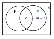
Suppose an experiment consists of \(n\) equally likely events. Further suppose that there are \(m\) elements in \(\mathrm{F}\), and \(c\) elements in \(\mathrm{E} \cap \mathrm{F}\), as shown in the following Venn diagram.

If the event \(\mathrm{F}\) has occurred, the set of all possible outcomes is no longer the entire sample space, but instead, the subset \(\mathrm{F}\). Therefore, we only look at the set \(\mathrm{F}\) and at nothing outside of \(\mathrm{F}\). Since \(\mathrm{F}\) has \(m\) elements, the denominator in the calculation of \(\mathrm{P(E | F)}\) is \(m\). We may think that the numerator for our conditional probability is the number of elements in \(\mathrm{E}\). But clearly we cannot consider the elements of \(\mathrm{E}\) that are not in \(\mathrm{F}\). We can only count the elements of \(\mathrm{E}\) that are in \(\mathrm{F}\), that is, the elements in \(\mathrm{E} \cap \mathrm{F}\). Therefore,
\[\mathrm{P}(\mathrm{E} | \mathrm{F})=\frac{\mathrm{c}}{\mathrm{m}} \nonumber \]
Dividing both the numerator and the denominator by \(n\), we get
\[\mathrm{P(E | F)}=\frac{c / n}{m / n} \nonumber \]
But \(c/n = \mathrm{P}(\mathrm{E} \cap \mathrm{F})\), and \(m/n = \mathrm{P}(\mathrm{F})\).
Substituting, we derive the following formula for \(\mathrm{P}(\mathrm{E} | \mathrm{F})\).
Conditional Probability Rule
For two events \(\mathrm{E}\) and \(\mathrm{F}\), the probability of "\(\mathrm{E}\) Given \(\mathrm{F}\)" is
\[\mathbf{P}(\mathbf{E} | \mathbf{F})=\frac{\mathbf{P}(\mathbf{E} \cap \mathbf{F})}{\mathbf{P}(\mathbf{F})} \nonumber \]
Example \(\PageIndex{4}\)
A single die is rolled. Use the above formula to find the conditional probability of obtaining an even number given that a number greater than three has shown.
Solution
Let \(\mathrm{E}\) be the event that an even number shows, and \(\mathrm{F}\) be the event that a number greater than three shows. We want \(\mathrm{P}(\mathrm{E} | \mathrm{F})\).
\(\mathrm{E} = {2, 4, 6}\) and \(\mathrm{F} = {4, 5, 6}\). Which implies, \(\mathrm{E} \cap \mathrm{F} = { 4, 6}\)
Therefore, \(\mathrm{P}(\mathrm{F})\) = 3/6, and \(\mathrm{P}(\mathrm{E} \cap \mathrm{F})\) = 2/6
\[P(E | F)=\frac{P(E \cap F)}{P(F)}=\frac{2 / 6}{3 / 6}=\frac{2}{3} \nonumber. \nonumber \]
Example \(\PageIndex{5}\)
The following table shows the distribution by gender of students at a community college who take public transportation and the ones who drive to school.
|
|
Male(M) |
Female(F) |
Total |
| Public Transportation(T) |
8 |
13 |
21 |
| Drive(D) |
39 |
40 |
79 |
| Total |
47 |
53 |
100 |
The events \(\mathrm{M}, \mathrm{F}, \mathrm{T}\), and \(\mathrm{D}\) are self explanatory. Find the following probabilities.
- \(\mathrm{P}(\mathrm{D} | \mathrm{M})\)
- \(\mathrm{P}(\mathrm{F} | \mathrm{D})\)
- \(\mathrm{P}(\mathrm{M} | \mathrm{T})\)
Solution 1
Conditional probabilities can often be found directly from a contingency table. If the condition corresponds to only one row or only one column in the table, then you can ignore the rest of the table and read the conditional probability directly from the row or column indicated by the condition.
- The condition is event \(\mathrm{M}\); we can look at only the “Male” column of the table and ignore the rest of the table: \(\mathrm{P}(\mathrm{D} | \mathrm{M})=\frac{39}{47}\).
- The condition is event \(\mathrm{D}\); we can look at only the “Drive” row of the table and ignore the rest of the table: \(\mathrm{P}(\mathrm{F} | \mathrm{D})=\frac{40}{79}\).
- The condition is event \(\mathrm{T}\); we can look at only the “Public Transportation” row of the table and ignore the rest of the table: \(\mathrm{P}(\mathrm{M} | \mathrm{T})=\frac{8}{21}\).
Solution 2
We use the conditional probability formula \(\mathrm{P}(\mathrm{E} | \mathrm{F})=\frac{\mathrm{P}(\mathrm{E} \cap \mathrm{F})}{\mathrm{P(F)}}\).
- \[P(D | M)=\frac{P(D \cap M)}{P(M)}=\frac{39 / 100}{47 / 100}=\frac{39}{47} \nonumber . \nonumber \]
- \[P(F | D)=\frac{P(F \cap D)}{P(D)}=\frac{40 / 100}{79 / 100}=\frac{40}{79} \nonumber . \nonumber \]
- \[\mathrm{P}(\mathrm{M} | \mathrm{T})=\frac{P(M \cap T)}{P(T)}=\frac{8 / 100}{21 / 100}=\frac{8}{21} \nonumber \]
Example \(\PageIndex{6}\)
Given \(\mathrm{P(E)}\) = .5, \(\mathrm{P}(\mathrm{F})\) = .7, and \(\mathrm{P}(\mathrm{E} \cap \mathrm{F})\) = .3. Find the following:
- \(\mathrm{P}(\mathrm{E} | \mathrm{F})\)
- \(\mathrm{P}(\mathrm{F} | \mathrm{E})\)
Solution
We use the conditional probability formula.
- \(P(E | F)=\frac{P(E \cap F)}{P(F)}=\frac{3}{7}=\frac{3}{7}\)
- \(P(F | E)=\frac{P(E \cap F)}{P(E)}=.3 / .5=3 / 5 \)
Example \(\PageIndex{7}\)
\(\mathrm{E}\) and \(\mathrm{F}\) are mutually exclusive events such that \(\mathrm{P(E)}\) = .4, \(\mathrm{P(F)}\) = .9. Find \(\mathrm{P(E | F)}\).
Solution
\(\mathrm{E}\) and \(\mathrm{F}\) are mutually exclusive, so \(\mathrm{P}(\mathrm{E} \cap \mathrm{F})\) = 0.
Therefore \(\mathrm{P}(\mathrm{E} | \mathrm{F})=\frac{\mathrm{P}(\mathrm{E} \cap \mathrm{F})}{\mathrm{P}(\mathrm{F})}=\frac{0}{9}=0\).
Example \(\PageIndex{8}\)
Given \(\mathrm{P}(\mathrm{F} | \mathrm{E})\) = .5, and \(\mathrm{P}(\mathrm{E} \cap \mathrm{F})\) = .3. Find \(\mathrm{P}(\mathrm{E})\).
Solution
Using the conditional probability formula \(\mathrm{P}(\mathrm{E} | \mathrm{F})=\frac{\mathrm{P}(\mathrm{E} \cap \mathrm{F})}{\mathrm{P}(\mathrm{F})}\), we get
\[\mathrm{P}(\mathrm{F} | \mathrm{E})=\frac{\mathrm{P}(\mathrm{E} \cap \mathrm{F})}{\mathrm{P}(\mathrm{E})} \nonumber \]
Substituting and solving:
\[.5=\frac{.3}{\mathrm{P}(\mathrm{E})} \quad \text { or } \quad \mathrm{P}(\mathrm{E})=3 / 5 \nonumber \]
Example \(\PageIndex{9}\)
In a family of three children, find the conditional probability of having two boys and a girl, given that the family has at least two boys.
Solution
Let event \(\mathrm{E}\) be that the family has two boys and a girl, and let \(\mathrm{F}\) be the probability that the family has at least two boys. We want \(\mathrm{P}(\mathrm{E} | \mathrm{F})\).
We list the sample space along with the events \(\mathrm{E}\) and \(\mathrm{F}\).
\begin{aligned}
&\mathrm{S}=\{\mathrm{BBB}, \mathrm{BBG}, \mathrm{BGB}, \mathrm{BGG}, \mathrm{GBB}, \mathrm{GBG}, \mathrm{GGB}, \mathrm{GGG}\}\\
&\mathrm{E}=\{\mathrm{BBG}, \mathrm{BGB}, \mathrm{GBB}\} \text { and } \mathrm{F}=\{\mathrm{BBB}, \mathrm{BBG}, \mathrm{BGB}, \mathrm{GBB}\}\\
&\mathrm{E} \cap \mathrm{F}=\{\mathrm{BBG}, \mathrm{BGB}, \mathrm{GBB}\}
\end{aligned}
Therefore, \(\mathrm{P}(\mathrm{F})\) = 4/8, and \(\mathrm{P}(\mathrm{E} \cap \mathrm{F})\) = 3/8, and
\[\mathrm{P}(\mathrm{E} | \mathrm{F})=\frac{\mathrm{P}(\mathrm{E} \cap \mathrm{F})}{\mathrm{P}(\mathrm{E})} =\frac{3/8}{4/8} =\frac{3}{4} \nonumber. \nonumber \]
Example \(\PageIndex{10}\)
At a community college 65% of the students subscribe to Amazon Prime, 50% subscribe to Netflix, and 20% subscribe to both. If a student is chosen at random, find the following probabilities:
- the student subscribes to Amazon Prime given that he subscribes to Netflix
- the student subscribes to Netflix given that he subscribes to Amazon Prime
Solution
Let \(\mathrm{A}\) be the event that the student subscribes to Amazon Prime, and \(\mathrm{N}\) be the event that the student subscribes to Netflix.
First identify the probabilities and events given in the problem.
\(\mathrm{P}\)(student subscribes to Amazon Prime) = \(\mathrm{P(A)}\) = 0.65
\(\mathrm{P}\)(student subscribes to Netflix) = \(\mathrm{P(N)}\) = 0.50
\(\mathrm{P}\)(student subscribes to both Amazon Prime and Netflix) = \(\mathrm{P(A \cap N)}\) = 0.20
Then use the conditional probability rule:
- \(\mathrm{P}(\mathrm{A} | \mathrm{N})=\frac{\mathrm{P}(\mathrm{A} \cap \mathrm{N})}{\mathrm{P}(\mathrm{N})} = \frac{.20}{.50} = \frac{2}{5}\)
- \(\mathrm{P}(\mathrm{N} | \mathrm{A})=\frac{\mathrm{P}(\mathrm{A} \cap \mathrm{N})}{\mathrm{P}(\mathrm{A})} = \frac{.20}{.65} = \frac{4}{13}\)


