2.12: Graphing Rational Functions

We’ve seen that the denominator of a rational function is never allowed to equal zero; division by zero is not defined. So, with rational functions, there are special values of the independent variable that are of particular importance. Now, it comes as no surprise that near values that make the denominator zero, rational functions exhibit special behavior, but here, we will also see that values that make the numerator zero sometimes create additional special behavior in rational functions.

We begin our discussion by focusing on the domain of a rational function.

The Domain of a Rational Function

When presented with a rational function of the form

\[f(x)=\frac{a_{0}+a_{1} x+a_{2} x^{2}+\cdots+a_{n} x^{n}}{b_{0}+b_{1} x+b_{2} x^{2}+\cdots+b_{m} x^{m}} \nonumber \]

the first thing we must do is identify the domain. Equivalently, we must identify the restrictions, values of the independent variable (usually x) that are not in the domain. To facilitate the search for restrictions, we should factor the denominator of the rational function (it won’t hurt to factor the numerator at this time as well, as we will soon see). Once the domain is established and the restrictions are identified, here are the pertinent facts.

Behavior of a Rational Function at Its Restrictions

A rational function can only exhibit one of two behaviors at a restriction (a value of the independent variable that is not in the domain of the rational function).

1. The graph of the rational function will have a vertical asymptote at the restricted value.
2. The graph will exhibit a “hole” at the restricted value.

In the next two examples, we will examine each of these behaviors. In this first example, we see a restriction that leads to a vertical asymptote.

Example \(\PageIndex{1}\)

Sketch the graph of \[f(x)=\frac{1}{x+2} \nonumber \]

Solution

The first step is to identify the domain. Note that x = −2 makes the denominator of f(x) = 1/(x + 2) equal to zero. Division by zero is undefined. Hence, x = −2 is not in the domain of f; that is, x = −2 is a restriction. Equivalently, the domain of f is \(\{x : x \neq-2\}\).

Now that we’ve identified the restriction, we can use the theory of Section 7.1 to shift the graph of y = 1/x two units to the left to create the graph of \(f(x) = 1/(x + 2)\), as shown in Figure \(\PageIndex{1}\).

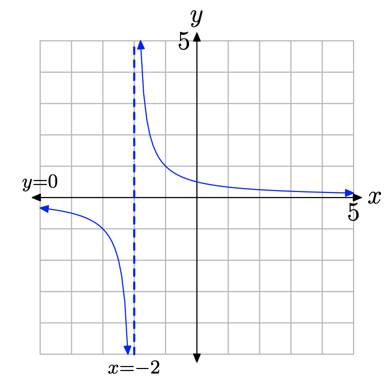Figure \(\PageIndex{1}\). The function f(x) = 1/(x + 2) has a restriction at x = −2. The graph of f has a vertical asymptote with equation x = −2.

The function f(x) = 1/(x + 2) has a restriction at x = −2 and the graph of f exhibits a vertical asymptote having equation x = −2.

It is important to note that although the restricted value x = −2 makes the denominator of f(x) = 1/(x + 2) equal to zero, it does not make the numerator equal to zero. We’ll soon have more to say about this observation.

Let’s look at an example of a rational function that exhibits a “hole” at one of its restricted values.

Example \(\PageIndex{2}\)

Sketch the graph of \[f(x)=\frac{x-2}{x^{2}-4} \nonumber \]

Solution

We highlight the first step.

Factor Numerators and Denominators

When working with rational functions, the first thing you should always do is factor both numerator and denominator of the rational function.

Following this advice, we factor both numerator and denominator of \(f(x) = (x − 2)/(x^2 − 4)\).

\[f(x)=\frac{x-2}{(x-2)(x+2)} \nonumber \]

It is easier to spot the restrictions when the denominator of a rational function is in factored form. Clearly, x = −2 and x = 2 will both make the denominator of f(x) = (x−2)/((x−2)(x+ 2)) equal to zero. Hence, x = −2 and x = 2 are restrictions of the rational function f.

Now that the restrictions of the rational function f are established, we proceed to the second step.

Reduce to Lowest Terms

After you establish the restrictions of the rational function, the second thing you should do is reduce the rational function to lowest terms.

Following this advice, we cancel common factors and reduce the rational function f(x) = (x − 2)/((x − 2)(x + 2)) to lowest terms, obtaining a new function,

\[g(x)=\frac{1}{x+2} \nonumber \]

The functions f(x) = (x − 2)/((x − 2)(x + 2)) and g(x) = 1/(x + 2) are not identical functions. They have different domains. The domain of f is \(D_{f}=\{x : x \neq-2,2\}\), but the domain of g is \(D_{g}=\{x : x \neq-2\}\). Hence, the only difference between the two functions occurs at x = 2. The number 2 is in the domain of g, but not in the domain of f.

We know what the graph of the function g(x) = 1/(x + 2) looks like. We drew this graph in Example \(\PageIndex{1}\) and we picture it anew in Figure \(\PageIndex{2}\).

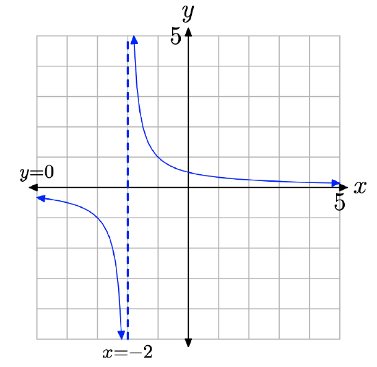Figure \(\PageIndex{2}\). The graph of g(x) = 1/(x + 2) exhibits a vertical asymptote at its restriction x = −2.

The difficulty we now face is the fact that we’ve been asked to draw the graph of f, not the graph of g. However, we know that the functions f and g agree at all values of x except x = 2. If we remove this value from the graph of g, then we will have the graph of f.

So, what point should we remove from the graph of g? We should remove the point that has an x-value equal to 2. Therefore, we evaluate the function g(x) = 1/(x + 2) at x = 2 and find \[g(2)=\frac{1}{2+2}=\frac{1}{4} \nonumber \]

Because g(2) = 1/4, we remove the point (2, 1/4) from the graph of g to produce the graph of f. The result is shown in Figure \(\PageIndex{3}\).

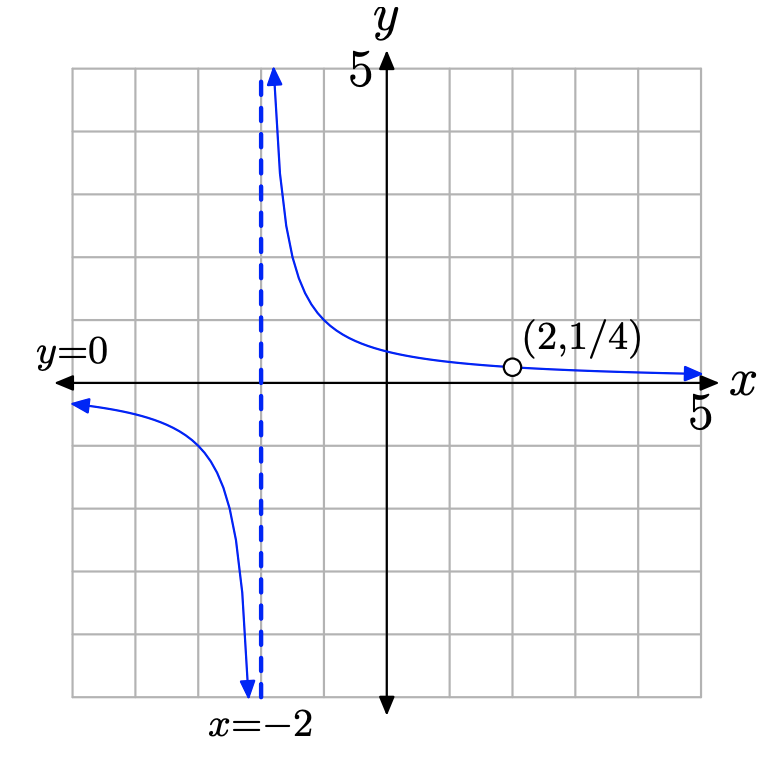Figure \(\PageIndex{3}\). The graph of f(x) = (x − 2)/((x − 2)(x + 2)) exhibits a vertical asymptote at its restriction x = −2 and a hole at its second restriction x = 2.

We pause to make an important observation. In Example \(\PageIndex{2}\), we started with the function

\[f(x)=\frac{x-2}{(x-2)(x+2)} \nonumber \]

which had restrictions at x = 2 and x = −2. After reducing, the function

\[g(x)=\frac{1}{x+2} \nonumber \]

no longer had a restriction at x = 2. The function g had a single restriction at x = −2. The result, as seen in Figure \(\PageIndex{3}\), was a vertical asymptote at the remaining restriction, and a hole at the restriction that “went away” due to cancellation. This leads us to the following procedure.

Asymptote or Hole?

To determine whether the graph of a rational function has a vertical asymptote or a hole at a restriction, proceed as follows:

1. Factor numerator and denominator of the original rational function f. Identify the restrictions of f.
2. Reduce the rational function to lowest terms, naming the new function g. Identify the restrictions of the function g.
3. Those restrictions of f that remain restrictions of the function g will introduce vertical asymptotes into the graph of f.
4. Those restrictions of f that are no longer restrictions of the function g will introduce “holes” into the graph of f. To determine the coordinates of the holes, substitute each restriction of f that is not a restriction of g into the function g to determine the y-value of the hole.

We now turn our attention to the zeros of a rational function.

The Zeros of a Rational Function

We’ve seen that division by zero is undefined. That is, if we have a fraction N/D, then D (the denominator) must not equal zero. Thus, 5/0, −15/0, and 0/0 are all undefined. On the other hand, in the fraction N/D, if N = 0 and \(D \neq 0\), then the fraction is equal to zero. For example, 0/5, 0/(−15), and 0\(/ \pi\) are all equal to zero.

Therefore, when working with an arbitrary rational function, such as

\[f(x)=\frac{a_{0}+a_{1} x+a_{2} x^{2}+\cdots+a_{n} x^{n}}{b_{0}+b_{1} x+b_{2} x^{2}+\cdots+b_{m} x^{m}} \nonumber \]

whatever value of x that will make the numerator zero without simultaneously making the denominator equal to zero will be a zero of the rational function f.

This discussion leads to the following procedure for identifying the zeros of a rational function.

Finding Zeros of Rational Functions

To determine the zeros of a rational function, proceed as follows.

1. Factor both numerator and denominator of the rational function f.
2. Identify the restrictions of the rational function f.
3. Identify the values of the independent variable (usually x) that make the numerator equal to zero.
4. The zeros of the rational function f will be those values of x that make the numerator zero but are not restrictions of the rational function f.

Let’s look at an example.

Example \(\PageIndex{3}\)

Find the zeros of the rational function defined by \[f(x)=\frac{x^{2}+3 x+2}{x^{2}-2 x-3} \nonumber \]

Solution

Factor numerator and denominator of the rational function f.

\[f(x)=\frac{(x+1)(x+2)}{(x+1)(x-3)} \nonumber \]

The values x = −1 and x = 3 make the denominator equal to zero and are restrictions.

Next, note that x = −1 and x = −2 both make the numerator equal to zero. However, x = −1 is also a restriction of the rational function f, so it will not be a zero of f. On the other hand, the value x = −2 is not a restriction and will be a zero of f.

Although we’ve correctly identified the zeros of f, it’s instructive to check the values of x that make the numerator of f equal to zero. If we substitute x = −1 into original function defined by equation (6), we find that

\[f(-1)=\frac{(-1)^{2}+3(-1)+2}{(-1)^{2}-2(-1)-3}=\frac{0}{0} \nonumber \]

is undefined. Hence, x = −1 is not a zero of the rational function f. The difficulty in this case is that x = −1 also makes the denominator equal to zero.

On the other hand, when we substitute x = −2 in the function defined by equation (6),

\[f(-2)=\frac{(-2)^{2}+3(-2)+2}{(-2)^{2}-2(-2)-3}=\frac{0}{5}=0 \nonumber \]

In this case, x = −2 makes the numerator equal to zero without making the denominator equal to zero. Hence, x = −2 is a zero of the rational function f.

It’s important to note that you must work with the original rational function, and not its reduced form, when identifying the zeros of the rational function.

Example \(\PageIndex{4}\)

Identify the zeros of the rational function \[f(x)=\frac{x^{2}-6 x+9}{x^{2}-9} \nonumber \]

Solution

Factor both numerator and denominator. \[f(x)=\frac{(x-3)^{2}}{(x+3)(x-3)} \nonumber \]

Note that x = −3 and x = 3 are restrictions. Further, the only value of x that will make the numerator equal to zero is x = 3. However, this is also a restriction. Hence, the function f has no zeros.

The point to make here is what would happen if you work with the reduced form of the rational function in attempting to find its zeros. Cancelling like factors leads to a new function,

\[g(x)=\frac{x-3}{x+3} \nonumber \]

Note that g has only one restriction, x = −3. Further, x = 3 makes the numerator of g equal to zero and is not a restriction. Hence, x = 3 is a zero of the function g, but it is not a zero of the function f.

This example demonstrates that we must identify the zeros of the rational function before we cancel common factors.

Drawing the Graph of a Rational Function

In this section we will use the zeros and asymptotes of the rational function to help draw the graph of a rational function. We will also investigate the end-behavior of rational functions. Let’s begin with an example.

Example \(\PageIndex{5}\)

Sketch the graph of the rational function \[f(x)=\frac{x+2}{x-3} \nonumber \]

Solution

First, note that both numerator and denominator are already factored. The function has one restriction, x = 3. Next, note that x = −2 makes the numerator of equation (9) zero and is not a restriction. Hence, x = −2 is a zero of the function. Recall that a function is zero where its graph crosses the horizontal axis. Hence, the graph of f will cross the x-axis at (−2, 0), as shown in Figure \(\PageIndex{4}\).

Note that the rational function (9) is already reduced to lowest terms. Hence, the restriction at x = 3 will place a vertical asymptote at x = 3, which is also shown in Figure \(\PageIndex{4}\).

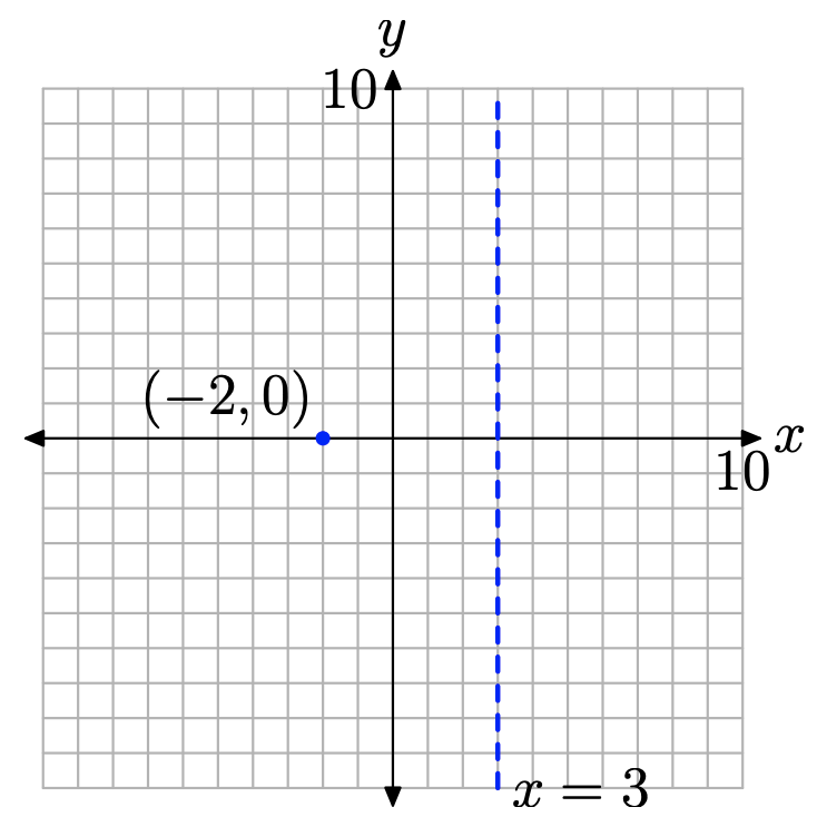Figure \(\PageIndex{4}\). Plot and label the x-intercept and vertical asymptote.

At this point, we know two things:

1. The graph will cross the x-axis at (−2, 0).
2. On each side of the vertical asymptote at x = 3, one of two things can happen. Either the graph will rise to positive infinity or the graph will fall to negative infinity.

To discover the behavior near the vertical asymptote, let’s plot one point on each side of the vertical asymptote, as shown in Figure \(\PageIndex{5}\).

Figure \(\PageIndex{5}\). Additional points help determine the behavior near the vertical asymptote.

Consider the right side of the vertical asymptote and the plotted point (4, 6) through which our graph must pass. As the graph approaches the vertical asymptote at x = 3, only one of two things can happen. Either the graph rises to positive infinity or the graph falls to negative infinity. However, in order for the latter to happen, the graph must first pass through the point (4, 6), then cross the x-axis between x = 3 and x = 4 on its descent to minus infinity. But we already know that the only x-intercept is at the point (2, 0), so this cannot happen. Hence, on the right, the graph must pass through the point (4, 6), then rise to positive infinity, as shown in Figure \(\PageIndex{6}\).

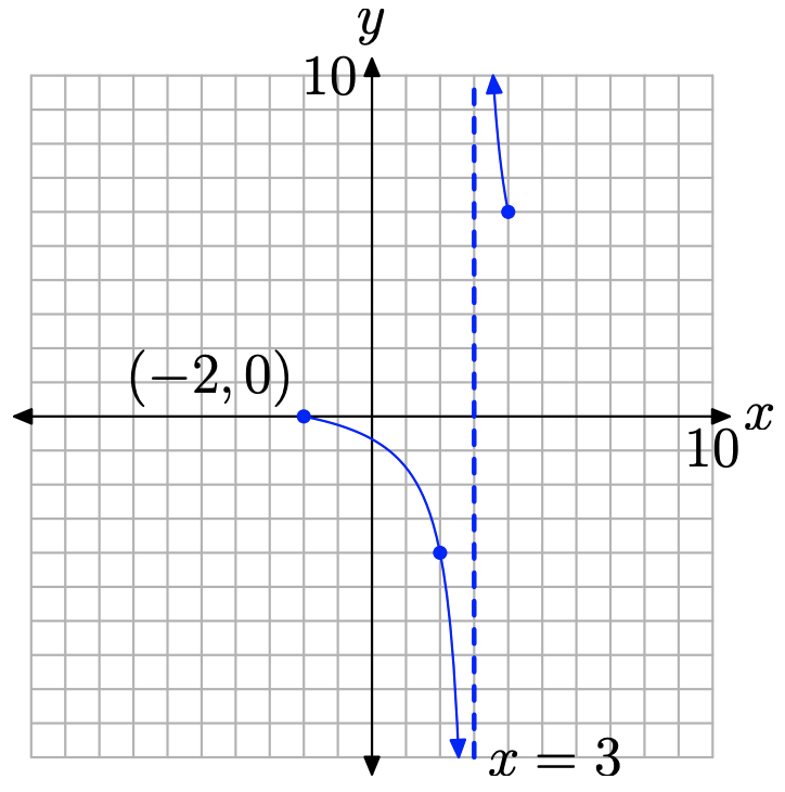Figure \(\PageIndex{6}\). Behavior near the vertical asymptote.

A similar argument holds on the left of the vertical asymptote at x = 3. The graph cannot pass through the point (2, −4) and rise to positive infinity as it approaches the vertical asymptote, because to do so would require that it cross the x-axis between x = 2 and x = 3. However, there is no x-intercept in this region available for this purpose. Hence, on the left, the graph must pass through the point (2, −4) and fall to negative infinity as it approaches the vertical asymptote at x = 3. This behavior is shown in Figure \(\PageIndex{6}\).

Finally, what about the end-behavior of the rational function? What happens to the graph of the rational function as x increases without bound? What happens when x decreases without bound? One simple way to answer these questions is to use a table to investigate the behavior numerically. The graphing calculator facilitates this task.

First, enter your function as shown in Figure \(\PageIndex{7}\)(a), then press 2nd TBLSET to open the window shown in Figure \(\PageIndex{7}\)(b). For what we are about to do, all of the settings in this window are irrelevant, save one. Make sure you use the arrow keys to highlight ASK for the Indpnt (independent) variable and press ENTER to select this option. Finally, select 2nd TABLE, then enter the x-values 10, 100, 1000, and 10000, pressing ENTER after each one.

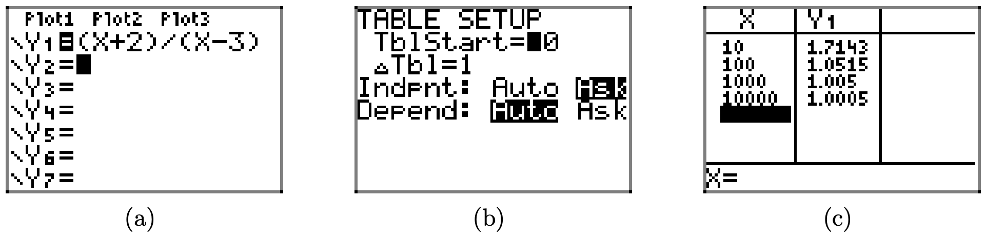Figure \(\PageIndex{7}\). Using the table feature of the graphing calculator to investigate the end-behavior as x approaches positive infinity.

Note the resulting y-values in the second column of the table (the Y1 column) in Figure \(\PageIndex{7}\)(c). As x is increasing without bound, the y-values are greater than 1, yet appear to be approaching the number 1. Therefore, as our graph moves to the extreme right, it must approach the horizontal asymptote at y = 1, as shown in Figure \(\PageIndex{9}\).

A similar effort predicts the end-behavior as x decreases without bound, as shown in the sequence of pictures in Figure \(\PageIndex{8}\). As x decreases without bound, the y-values are less than 1, but again approach the number 1, as shown in Figure \(\PageIndex{8}\)(c).

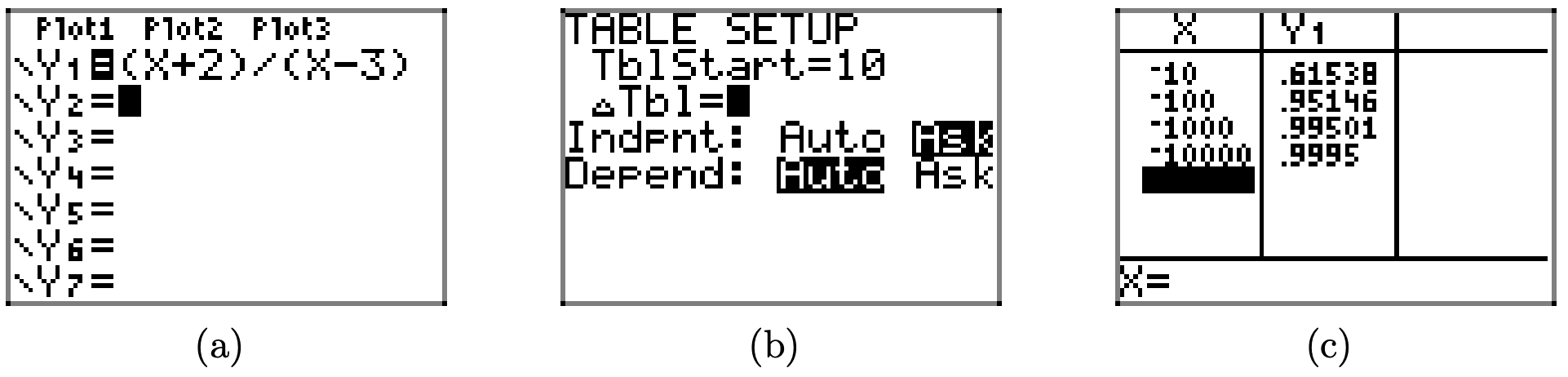Figure \(\PageIndex{8}\). Using the table feature of the graphing calculator to investigate the end-behavior as x approaches negative infinity.

The evidence in Figure \(\PageIndex{8}\)(c) indicates that as our graph moves to the extreme left, it must approach the horizontal asymptote at y = 1, as shown in Figure \(\PageIndex{9}\).

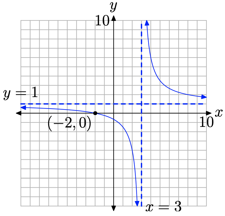Figure \(\PageIndex{9}\). The graph approaches the horizontal asymptote y = 1 at the extreme right- and left-ends.

What kind of job will the graphing calculator do with the graph of this rational function? In Figure \(\PageIndex{10}\)(a), we enter the function, adjust the window parameters as shown in Figure \(\PageIndex{10}\)(b), then push the GRAPH button to produce the result in Figure \(\PageIndex{10}\)(c).

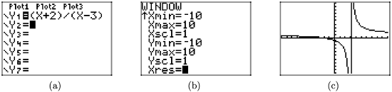Figure \(\PageIndex{10}\). Drawing the graph of the rational function with the graphing calculator.

As was discussed in the first section, the graphing calculator manages the graphs of “continuous” functions extremely well, but has difficulty drawing graphs with discontinuities. In the case of the present rational function, the graph “jumps” from negative

infinity to positive infinity across the vertical asymptote x = 3. The calculator knows only one thing: plot a point, then connect it to the previously plotted point with a line segment. Consequently, it does what it is told, and “connects” infinities when it shouldn’t.

However, if we have prepared in advance, identifying zeros and vertical asymptotes, then we can interpret what we see on the screen in Figure \(\PageIndex{10}\)(c), and use that information to produce the correct graph that is shown in Figure \(\PageIndex{9}\). We can even add the horizontal asymptote to our graph, as shown in the sequence in Figure \(\PageIndex{11}\).

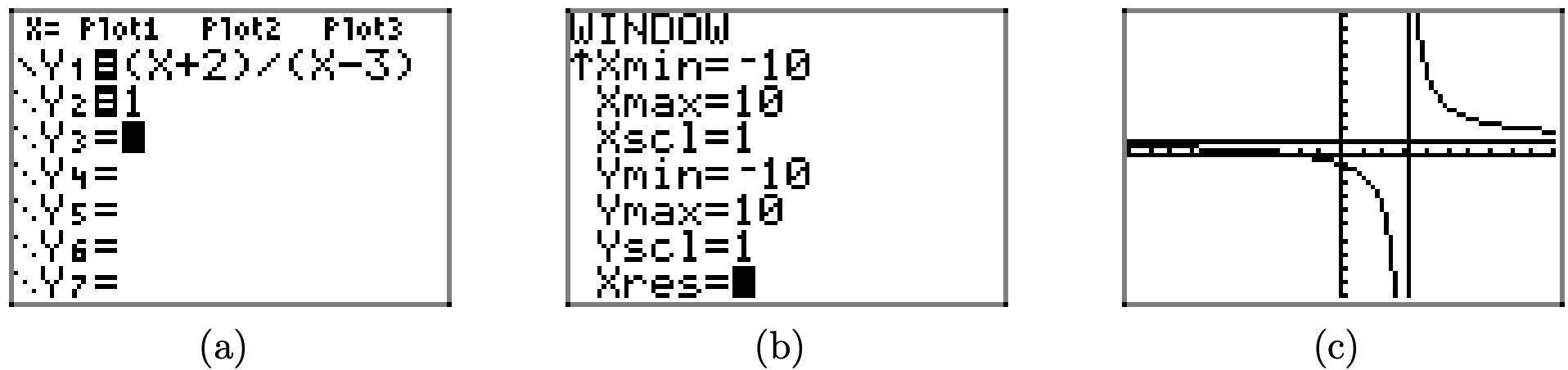Figure \(\PageIndex{11}\). Adding a suspected horizontal asymptote.

This is an appropriate point to pause and summarize the steps required to draw the graph of a rational function.

Procedure for Graphing Rational Functions

Consider the rational function \[f(x)=\frac{a_{0}+a_{1} x+a_{2} x^{2}+\cdots+a_{n} x^{n}}{b_{0}+b_{1} x+b_{2} x^{2}+\cdots+b_{m} x^{m}} \nonumber \]. To draw the graph of this rational function, proceed as follows:

1. Factor the numerator and denominator of the rational function f.
2. Identify the domain of the rational function f by listing each restriction, values of the independent variable (usually x) that make the denominator equal to zero.
3. Identify the values of the independent variable that make the numerator of f equal to zero and are not restrictions. These are the zeros of f and they provide the x-coordinates of the x-intercepts of the graph of the rational function. Plot these intercepts on a coordinate system and label them with their coordinates.
4. Cancel common factors to reduce the rational function to lowest terms. − The restrictions of f that remain restrictions of this reduced form will place vertical asymptotes in the graph of f. Draw the vertical asymptotes on your coordinate system as dashed lines and label them with their equations. − The restrictions of f that are not restrictions of the reduced form will place “holes” in the graph of f. We’ll deal with the holes in step 8 of this procedure.
5. To determine the behavior near each vertical asymptote, calculate and plot one point on each side of each vertical asymptote.
6. To determine the end-behavior of the given rational function, use the table capability of your calculator to determine the limit of the function as x approaches positive and/or negative infinity (as we did in the sequences shown in Figure \(\PageIndex{7}\) and Figure \(\PageIndex{8}\)). This determines the horizontal asymptote. Sketch the horizontal asymptote as a dashed line on your coordinate system and label it with its equation.
7. Draw the graph of the rational function.
8. If you determined that a restriction was a “hole,” use the restriction and the reduced form of the rational function to determine the y-value of the “hole.” Draw an open circle at this position to represent the “hole” and label the “hole” with its coordinates.
9. Finally, use your calculator to check the validity of your result.

Let’s look at another example.

Example \(\PageIndex{6}\)

Sketch the graph of the rational function \[f(x)=\frac{x-2}{x^{2}-3 x-4} \nonumber \]

Solution

We will follow the outline presented in the Procedure for Graphing Rational Functions.

Step 1: First, factor both numerator and denominator.

\[f(x)=\frac{x-2}{(x+1)(x-4)} \nonumber \]

Step 2: Thus, f has two restrictions, x = −1 and x = 4. That is, the domain of f is \(D_{f}=\{s : x \neq-1,4\}\).

Step 3: The numerator of equation (12) is zero at x = 2 and this value is not a restriction. Thus, 2 is a zero of f and (2, 0) is an x-intercept of the graph of f, as shown in Figure \(\PageIndex{12}\).

Step 4: Note that the rational function is already reduced to lowest terms (if it weren’t, we’d reduce at this point). Note that the restrictions x = −1 and x = 4 are still restrictions of the reduced form. Hence, these are the locations and equations of the vertical asymptotes, which are also shown in Figure \(\PageIndex{12}\).

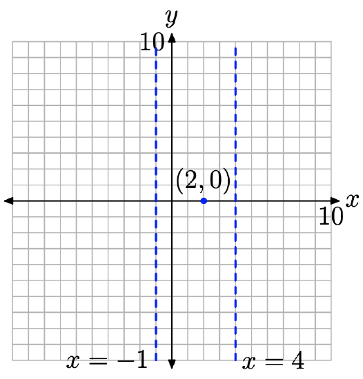Figure \(\PageIndex{12}\). Plot the x-intercepts and draw the vertical asymptotes.

All of the restrictions of the original function remain restrictions of the reduced form. Therefore, there will be no “holes” in the graph of f.

Step 5: Plot points to the immediate right and left of each asymptote, as shown in Figure \(\PageIndex{13}\). These additional points completely determine the behavior of the graph near each vertical asymptote. For example, consider the point (5, 1/2) to the immediate right of the vertical asymptote x = 4 in Figure \(\PageIndex{13}\). Because there is no x-intercept between x = 4 and x = 5, and the graph is already above the x-axis at the point (5, 1/2), the graph is forced to increase to positive infinity as it approaches the vertical asymptote x = 4. Similar comments are in order for the behavior on each side of each vertical asymptote.

Step 6: Use the table utility on your calculator to determine the end-behavior of the rational function as x decreases and/or increases without bound. To determine the end-behavior as x goes to infinity (increases without bound), enter the equation in your calculator, as shown in Figure \(\PageIndex{14}\)(a). Select 2nd TBLSET and highlight ASK for the independent variable. Select 2nd TABLE, then enter 10, 100, 1000, and 10000, as shown in Figure \(\PageIndex{14}\)(c).

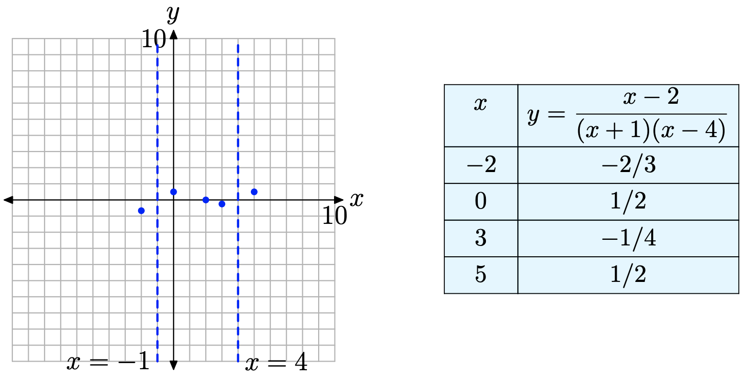Figure \(\PageIndex{13}\). Additional points help determine the behavior near the vertical asymptote. 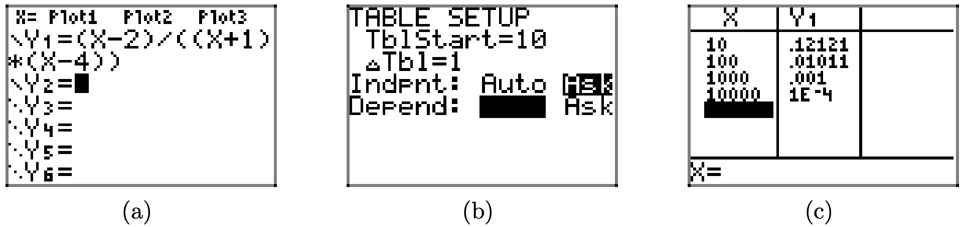Figure \(\PageIndex{14}\). Examining end-behavior as x approaches positive infinity

If you examine the y-values in Figure \(\PageIndex{14}\)(c), you see that they are heading towards zero (1e-4 means \(1 \times 10^{-4}\), which equals 0.0001). This implies that the line y = 0 (the x-axis) is acting as a horizontal asymptote.

You can also determine the end-behavior as x approaches negative infinity (decreases without bound), as shown in the sequence in Figure \(\PageIndex{15}\). The result in Figure \(\PageIndex{15}\)(c) provides clear evidence that the y-values approach zero as x goes to negative infinity. Again, this makes y = 0 a horizontal asymptote.

Figure \(\PageIndex{15}\). Examining end-behavior as x approaches negative infinity

Add the horizontal asymptote y = 0 to the image in Figure \(\PageIndex{13}\).

Step 7: We can use all the information gathered to date to draw the image shown in Figure \(\PageIndex{16}\).

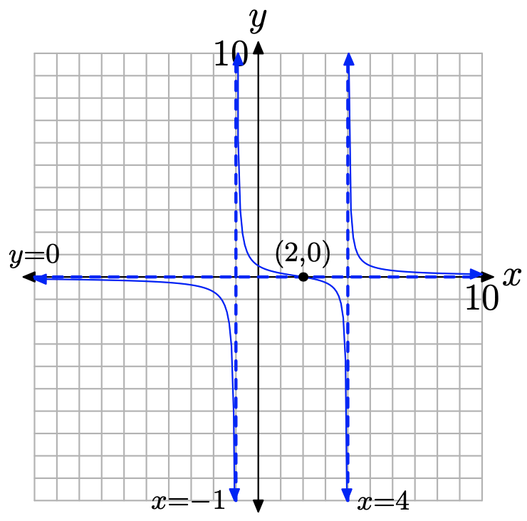Figure \(\PageIndex{16}\). The completed graph runs up against vertical and horizontal asymptotes and crosses the x-axis at the zero of the function.

Step 8: As stated above, there are no “holes” in the graph of f.

Step 9: Use your graphing calculator to check the validity of your result. Note how the graphing calculator handles the graph of this rational function in the sequence in Figure \(\PageIndex{17}\). The image in Figure \(\PageIndex{17}\)(c) is nowhere near the quality of the image we have in Figure \(\PageIndex{16}\), but there is enough there to intuit the actual graph if you prepare properly in advance (zeros, vertical asymptotes, end-behavior analysis, etc.).

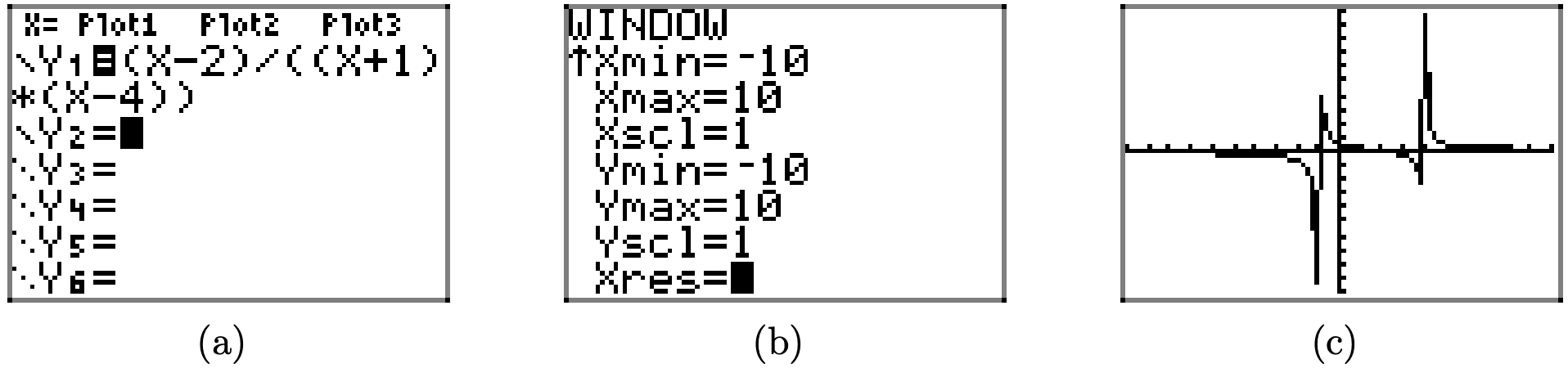Figure \(\PageIndex{17}\). The user of the graphing calculator must decipher the image in the calculator’s view screen.

Exercise

For rational functions Exercises 1-20, follow the Procedure for Graphing Rational Functions in the narrative, performing each of the following tasks.

1. Set up a coordinate system on graph paper. Label and scale each axis. Remember to draw all lines with a ruler.
2. Perform each of the nine steps listed in the Procedure for Graphing Rational Functions in the narrative.

Exercise \(\PageIndex{1}\)

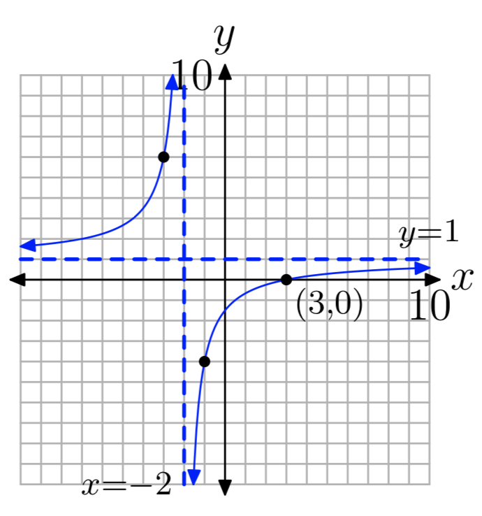
\(f(x) = \frac{x−3}{x+2}\)

Answer

Exercise \(\PageIndex{2}\)

\(f(x) = \frac{x+2}{x−4}\)

Exercise \(\PageIndex{3}\)

\(f(x) = \frac{5−x}{x+1}\)

Answer

Exercise \(\PageIndex{4}\)

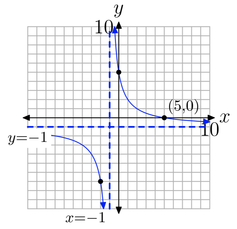
\(f(x) = \frac{x+2}{4−x}\)

Exercise \(\PageIndex{5}\)

\(f(x) = \frac{2x−5}{x+1}\)

Answer

Exercise \(\PageIndex{6}\)

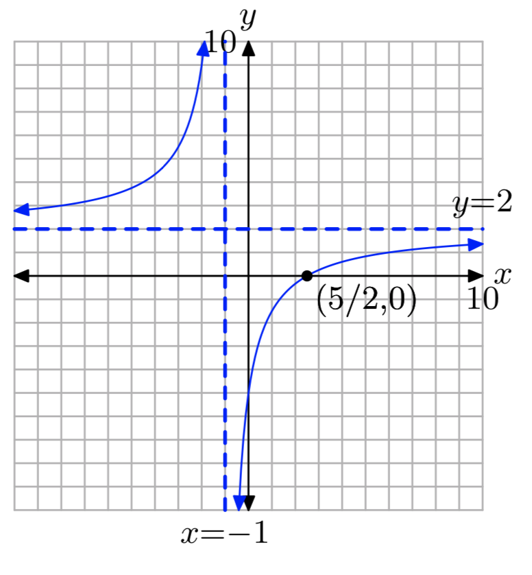
\(f(x) = \frac{2x+5}{3−x}\)

Exercise \(\PageIndex{7}\)

\(f(x) = \frac{x+2}{x^2−2x−3}\)

Answer

Exercise \(\PageIndex{8}\)

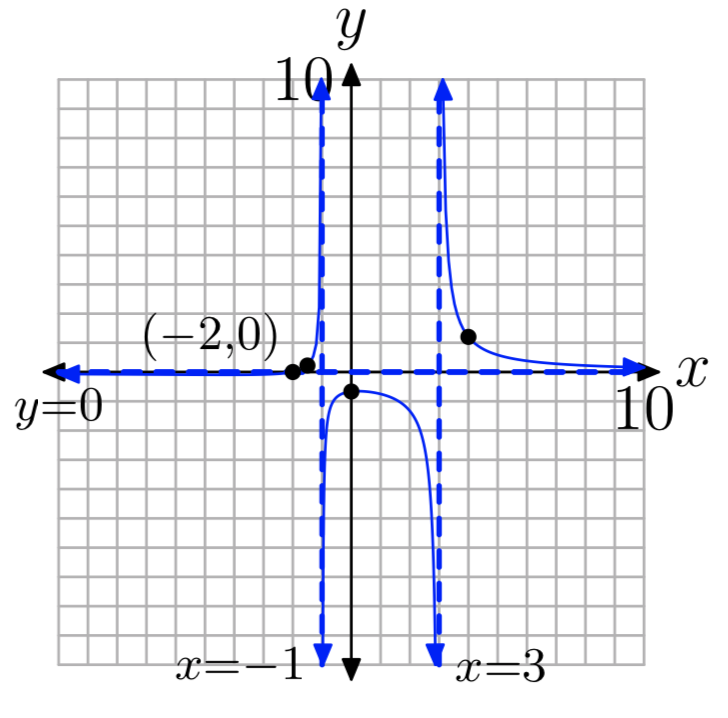
\(f(x) = \frac{x−3}{x^2−3x−4}\)

Exercise \(\PageIndex{9}\)

\(f(x) = \frac{x+1}{x^2+x−2}\)

Answer

Exercise \(\PageIndex{10}\)

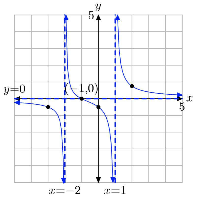
\(f(x) = \frac{x−1}{x^2−x−2}\)

Exercise \(\PageIndex{11}\)

\(f(x) = \frac{x^2−2x}{x^2+x−2}\)

Answer

Exercise \(\PageIndex{12}\)

\(f(x) = \frac{x^2−2x}{x^2−2x−8}\)

Exercise \(\PageIndex{13}\)

\(f(x) = \frac{2x^2−2x−4}{x^2−x−12}\)

Answer

Exercise \(\PageIndex{14}\)

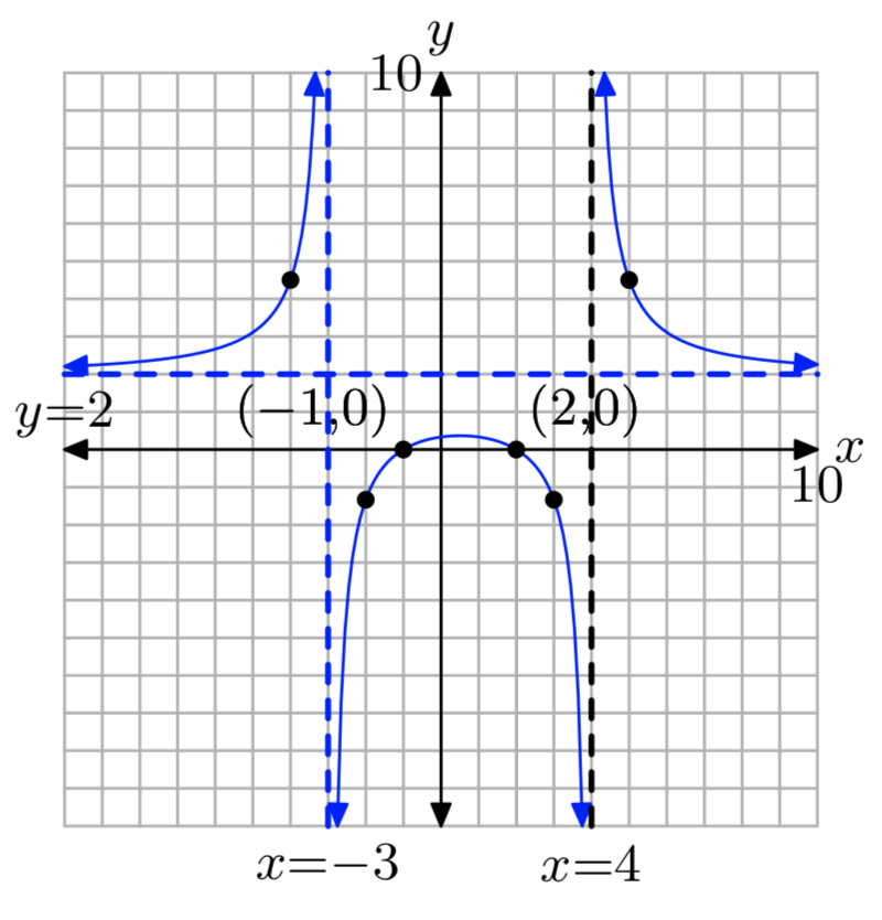
\(f(x) = \frac{8x−2x^2}{x^2−x−6}\)

Exercise \(\PageIndex{15}\)

\(f(x) = \frac{x−3}{x^2−5x+6}\)

Answer

Exercise \(\PageIndex{16}\)

\(f(x) = \frac{2x−4}{x^2−x−2}\)

Exercise \(\PageIndex{17}\)

\(f(x) = \frac{2x^2−x−6}{x^2−2x}\)

Answer

Exercise \(\PageIndex{18}\)

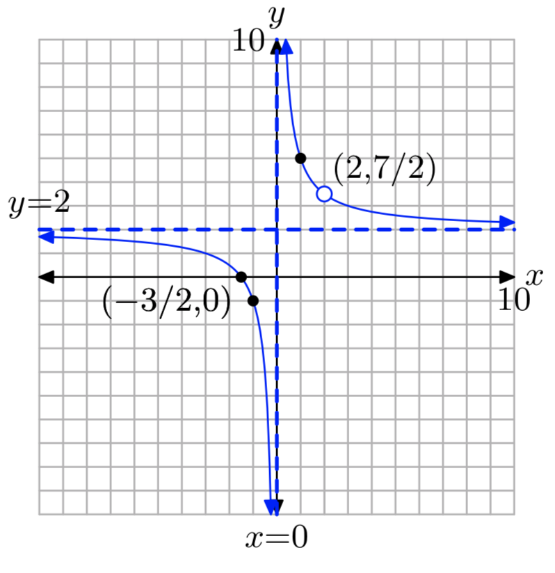
\(f(x) = \frac{2x^2−x−6}{x^2−2x}\)

Exercise \(\PageIndex{19}\)

\(f(x) = \frac{4+2x−2x^2}{x^2+4x+3}\)

Answer

Exercise \(\PageIndex{20}\)

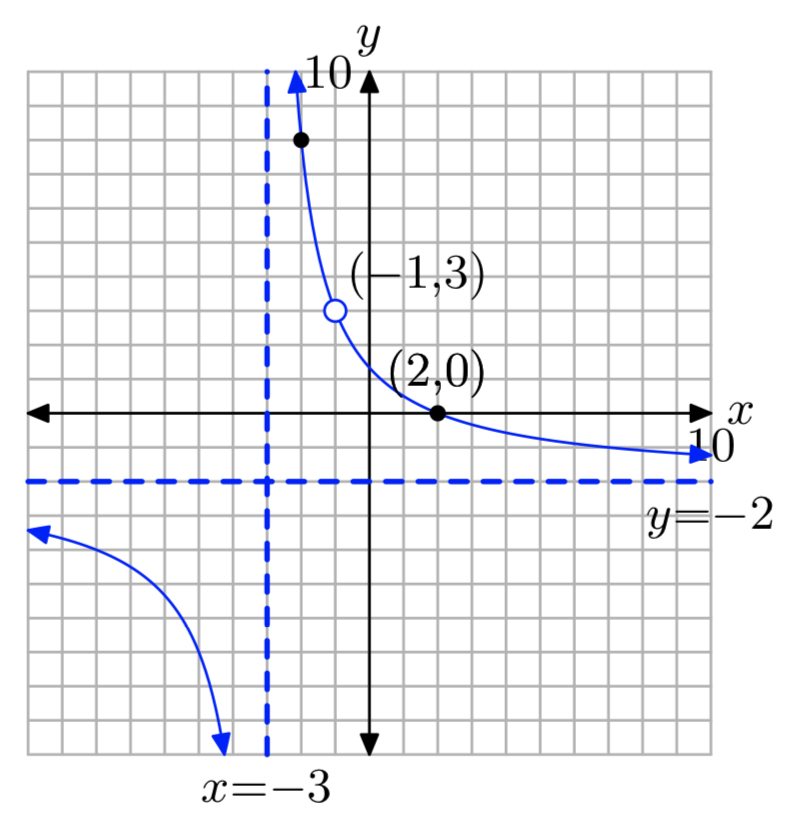
\(f(x) = \frac{3x^2−6x−9}{1−x^2}\)

In Exercises 21-28, find the coordinates of the x-intercept(s) of the graph of the given rational function.

Exercise \(\PageIndex{21}\)

\(f(x) = \frac{81−x^2}{x^2+10x+9}\)

Answer

(9, 0)

Exercise \(\PageIndex{22}\)

\(f(x) = \frac{x−x^2}{x^2+5x−6}\)

Exercise \(\PageIndex{23}\)

\(f(x) = \frac{x^2−x−12}{x^2+2x−3}\)

Answer

(4, 0)

Exercise \(\PageIndex{24}\)

\(f(x) = \frac{x^2−81}{x^2−4x−45}\)

Exercise \(\PageIndex{25}\)

\(f(x) = \frac{6x−18}{x^2−7x+12}\)

Answer

no x-intercepts

Exercise \(\PageIndex{26}\)

\(f(x) = \frac{4x+36}{x^2+15x+54}\)

Exercise \(\PageIndex{27}\)

\(f(x) = \frac{x^2−9x+14}{x^2−2x}\)

Answer

(7, 0)

Exercise \(\PageIndex{28}\)

\(f(x) = \frac{x^2−5x−36}{x^2−9x+20}\)

In Exercises 29-36, find the equations of all vertical asymptotes.

Exercise \(\PageIndex{29}\)

\(f(x) = \frac{x^2−7x}{x^2−2x}\)

Answer

x = 2

Exercise \(\PageIndex{30}\)

\(f(x) = \frac{x^2+4x−45}{3x+27}\)

Exercise \(\PageIndex{31}\)

\(f(x) = \frac{x^2−6x+8}{x^2−16}\)

Answer

x = −4

Exercise \(\PageIndex{32}\)

\(f(x) = \frac{x^2−11x+18}{2x−x^2}\)

Exercise \(\PageIndex{33}\)

\(f(x) = \frac{x^2+x−12}{−4x+12}\)

Answer

no vertical asymptotes

Exercise \(\PageIndex{34}\)

\(f(x) = \frac{x^2−3x−54}{9x−x^2}\)

Exercise \(\PageIndex{35}\)

\(f(x) = \frac{16−x^2}{x^2+7x+12}\)

Answer

x = −3

Exercise \(\PageIndex{36}\)

\(f(x) = \frac{x^2−11x+30}{−8x+48}\)

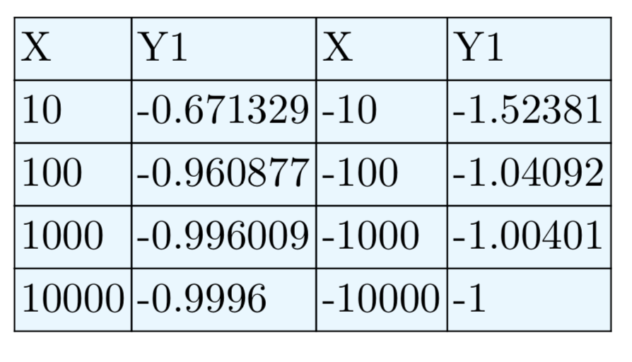
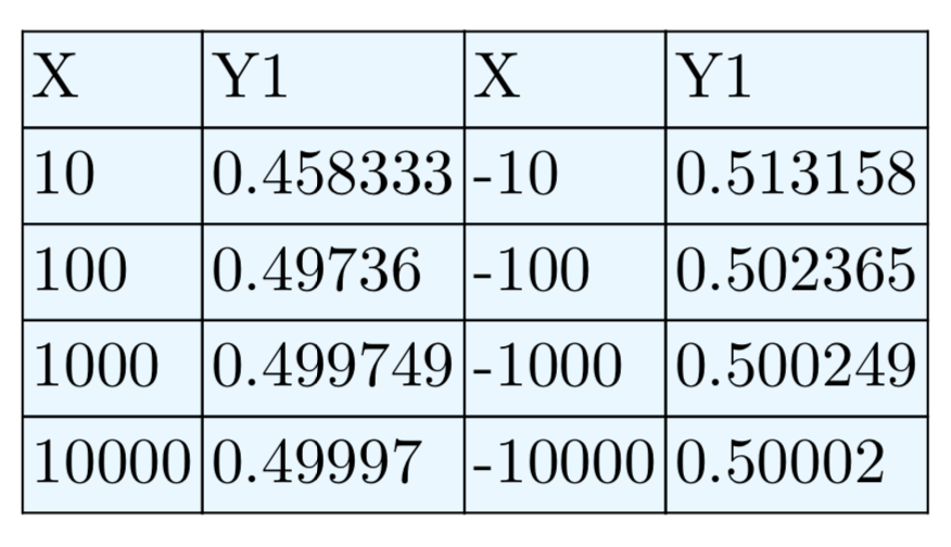
In Exercises 37-42, use a graphing calculator to determine the behavior of the given rational function as x approaches both positive and negative infinity by performing the following tasks:

1. Load the rational function into the Y=menu of your calculator.
2. Use the TABLE feature of your calculator to determine the value of f(x) for x = 10, 100, 1000, and 10000. Record these results on your homework in table form.
3. Use the TABLE feature of your calculator to determine the value of f(x) for x = −10, −100, −1000, and −10000. Record these results on your home- work in table form.
4. Use the results of your tabular exploration to determine the equation of the horizontal asymptote.

Exercise \(\PageIndex{37}\)

\(f(x) = \frac{2x+3}{x−8}\)

Answer

Horizontal asymptote at y = 2.

Exercise \(\PageIndex{38}\)

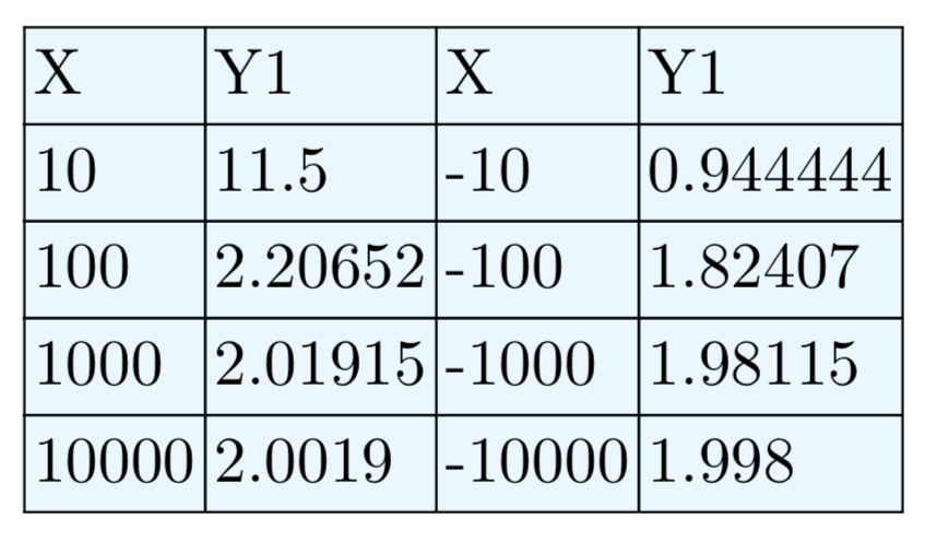
\(f(x) = \frac{4−3x}{x+2}\)

Exercise \(\PageIndex{39}\)

\(f(x) = \frac{4−x^2}{x^2+4x+3}\)

Answer

Horizontal asymptote at y = −1.

Exercise \(\PageIndex{40}\)

\(f(x) = \frac{10−2x^2}{x^2−4}\)

Exercise \(\PageIndex{41}\)

\(f(x) = \frac{x^2−2x−3}{2x^2−3x−2}\)

Answer

Horizontal asymptote at \(y = \frac{1}{2}\).

Exercise \(\PageIndex{42}\)

\(f(x) = \frac{2x^2−3x−5}{x^2−x−6}\)

In Exercises 43-48, use a purely analytical method to determine the domain of the given rational function. Describe the domain using set-builder notation.

Exercise \(\PageIndex{43}\)

\(f(x) = \frac{x^2−5x−6}{−9x−9}\)

Answer

Domain = {x: \(x \ne −1\)}

Exercise \(\PageIndex{44}\)

\(f(x) = \frac{x^2+4x+3}{x^2−5x−6}\)

Exercise \(\PageIndex{45}\)

\(f(x) = \frac{x^2+5x−24}{x^2−3x}\)

Answer

Domain = {x: \(x \ne 3, 0\)}

Exercise \(\PageIndex{46}\)

\(f(x) = \frac{x^2−3x−4}{x^2−5x−6}\)

Exercise \(\PageIndex{47}\)

\(f(x) = \frac{x^2−4x+3}{x−x^2}\)

Answer

Domain = {x: \(x \ne 0, 1\)}

Exercise \(\PageIndex{48}\)

\(f(x) = \frac{x^2−4}{x^2−9x+14}\)