4.7: Putting it All Together
- Page ID
- 22044
\( \newcommand{\vecs}[1]{\overset { \scriptstyle \rightharpoonup} {\mathbf{#1}} } \)
\( \newcommand{\vecd}[1]{\overset{-\!-\!\rightharpoonup}{\vphantom{a}\smash {#1}}} \)
\( \newcommand{\id}{\mathrm{id}}\) \( \newcommand{\Span}{\mathrm{span}}\)
( \newcommand{\kernel}{\mathrm{null}\,}\) \( \newcommand{\range}{\mathrm{range}\,}\)
\( \newcommand{\RealPart}{\mathrm{Re}}\) \( \newcommand{\ImaginaryPart}{\mathrm{Im}}\)
\( \newcommand{\Argument}{\mathrm{Arg}}\) \( \newcommand{\norm}[1]{\| #1 \|}\)
\( \newcommand{\inner}[2]{\langle #1, #2 \rangle}\)
\( \newcommand{\Span}{\mathrm{span}}\)
\( \newcommand{\id}{\mathrm{id}}\)
\( \newcommand{\Span}{\mathrm{span}}\)
\( \newcommand{\kernel}{\mathrm{null}\,}\)
\( \newcommand{\range}{\mathrm{range}\,}\)
\( \newcommand{\RealPart}{\mathrm{Re}}\)
\( \newcommand{\ImaginaryPart}{\mathrm{Im}}\)
\( \newcommand{\Argument}{\mathrm{Arg}}\)
\( \newcommand{\norm}[1]{\| #1 \|}\)
\( \newcommand{\inner}[2]{\langle #1, #2 \rangle}\)
\( \newcommand{\Span}{\mathrm{span}}\) \( \newcommand{\AA}{\unicode[.8,0]{x212B}}\)
\( \newcommand{\vectorA}[1]{\vec{#1}} % arrow\)
\( \newcommand{\vectorAt}[1]{\vec{\text{#1}}} % arrow\)
\( \newcommand{\vectorB}[1]{\overset { \scriptstyle \rightharpoonup} {\mathbf{#1}} } \)
\( \newcommand{\vectorC}[1]{\textbf{#1}} \)
\( \newcommand{\vectorD}[1]{\overrightarrow{#1}} \)
\( \newcommand{\vectorDt}[1]{\overrightarrow{\text{#1}}} \)
\( \newcommand{\vectE}[1]{\overset{-\!-\!\rightharpoonup}{\vphantom{a}\smash{\mathbf {#1}}}} \)
\( \newcommand{\vecs}[1]{\overset { \scriptstyle \rightharpoonup} {\mathbf{#1}} } \)
\( \newcommand{\vecd}[1]{\overset{-\!-\!\rightharpoonup}{\vphantom{a}\smash {#1}}} \)
\(\newcommand{\avec}{\mathbf a}\) \(\newcommand{\bvec}{\mathbf b}\) \(\newcommand{\cvec}{\mathbf c}\) \(\newcommand{\dvec}{\mathbf d}\) \(\newcommand{\dtil}{\widetilde{\mathbf d}}\) \(\newcommand{\evec}{\mathbf e}\) \(\newcommand{\fvec}{\mathbf f}\) \(\newcommand{\nvec}{\mathbf n}\) \(\newcommand{\pvec}{\mathbf p}\) \(\newcommand{\qvec}{\mathbf q}\) \(\newcommand{\svec}{\mathbf s}\) \(\newcommand{\tvec}{\mathbf t}\) \(\newcommand{\uvec}{\mathbf u}\) \(\newcommand{\vvec}{\mathbf v}\) \(\newcommand{\wvec}{\mathbf w}\) \(\newcommand{\xvec}{\mathbf x}\) \(\newcommand{\yvec}{\mathbf y}\) \(\newcommand{\zvec}{\mathbf z}\) \(\newcommand{\rvec}{\mathbf r}\) \(\newcommand{\mvec}{\mathbf m}\) \(\newcommand{\zerovec}{\mathbf 0}\) \(\newcommand{\onevec}{\mathbf 1}\) \(\newcommand{\real}{\mathbb R}\) \(\newcommand{\twovec}[2]{\left[\begin{array}{r}#1 \\ #2 \end{array}\right]}\) \(\newcommand{\ctwovec}[2]{\left[\begin{array}{c}#1 \\ #2 \end{array}\right]}\) \(\newcommand{\threevec}[3]{\left[\begin{array}{r}#1 \\ #2 \\ #3 \end{array}\right]}\) \(\newcommand{\cthreevec}[3]{\left[\begin{array}{c}#1 \\ #2 \\ #3 \end{array}\right]}\) \(\newcommand{\fourvec}[4]{\left[\begin{array}{r}#1 \\ #2 \\ #3 \\ #4 \end{array}\right]}\) \(\newcommand{\cfourvec}[4]{\left[\begin{array}{c}#1 \\ #2 \\ #3 \\ #4 \end{array}\right]}\) \(\newcommand{\fivevec}[5]{\left[\begin{array}{r}#1 \\ #2 \\ #3 \\ #4 \\ #5 \\ \end{array}\right]}\) \(\newcommand{\cfivevec}[5]{\left[\begin{array}{c}#1 \\ #2 \\ #3 \\ #4 \\ #5 \\ \end{array}\right]}\) \(\newcommand{\mattwo}[4]{\left[\begin{array}{rr}#1 \amp #2 \\ #3 \amp #4 \\ \end{array}\right]}\) \(\newcommand{\laspan}[1]{\text{Span}\{#1\}}\) \(\newcommand{\bcal}{\cal B}\) \(\newcommand{\ccal}{\cal C}\) \(\newcommand{\scal}{\cal S}\) \(\newcommand{\wcal}{\cal W}\) \(\newcommand{\ecal}{\cal E}\) \(\newcommand{\coords}[2]{\left\{#1\right\}_{#2}}\) \(\newcommand{\gray}[1]{\color{gray}{#1}}\) \(\newcommand{\lgray}[1]{\color{lightgray}{#1}}\) \(\newcommand{\rank}{\operatorname{rank}}\) \(\newcommand{\row}{\text{Row}}\) \(\newcommand{\col}{\text{Col}}\) \(\renewcommand{\row}{\text{Row}}\) \(\newcommand{\nul}{\text{Nul}}\) \(\newcommand{\var}{\text{Var}}\) \(\newcommand{\corr}{\text{corr}}\) \(\newcommand{\len}[1]{\left|#1\right|}\) \(\newcommand{\bbar}{\overline{\bvec}}\) \(\newcommand{\bhat}{\widehat{\bvec}}\) \(\newcommand{\bperp}{\bvec^\perp}\) \(\newcommand{\xhat}{\widehat{\xvec}}\) \(\newcommand{\vhat}{\widehat{\vvec}}\) \(\newcommand{\uhat}{\widehat{\uvec}}\) \(\newcommand{\what}{\widehat{\wvec}}\) \(\newcommand{\Sighat}{\widehat{\Sigma}}\) \(\newcommand{\lt}{<}\) \(\newcommand{\gt}{>}\) \(\newcommand{\amp}{&}\) \(\definecolor{fillinmathshade}{gray}{0.9}\)So, we've spend a lot of time going over different distributions. Why? Because they can answer research questions!
Standard Normal Curve
This is where it all comes together! What we can start doing with these distributions is comparing them. This might not sound like much, but it's the foundation of statistics, and allows us to answer research questions and test hypotheses.
- Probability Distributions: I know that I can make predictions from probability distributions. I can use probability distributions to understand the likelihood of specific events happening.
- Law of Large Numbers: I know through the Law of Large Numbers that enough of samples, their scores will be normally distributed (with all of the important characteristics that includes).
- Central Limit Theorem: I know through the Central Limit Theorem that if I get the means of enough samples, that the sampling distribution of means will be normally distributed.
- Standard Normal Distributions: I know that the mean is converted to always be zero, and the standard deviation is standardized to always be 1 in Standard Normal Distributions.
In Figure \(\PageIndex{1}\), the x-axis corresponds to the value of some variable, and the y-axis tells us something about how likely we are to observe that value. Notice that the y-axis is labeled “Probability Density” and not “Probability”. There is a subtle and somewhat frustrating characteristic of continuous distributions that makes the y-axis behave a bit oddly: the height of the curve here isn’t actually the probability of observing a particular x value. On the other hand, it is true that the heights of the curve tells you which x values are more likely (the higher ones!). This will be discussed in the Continuous Variable section.
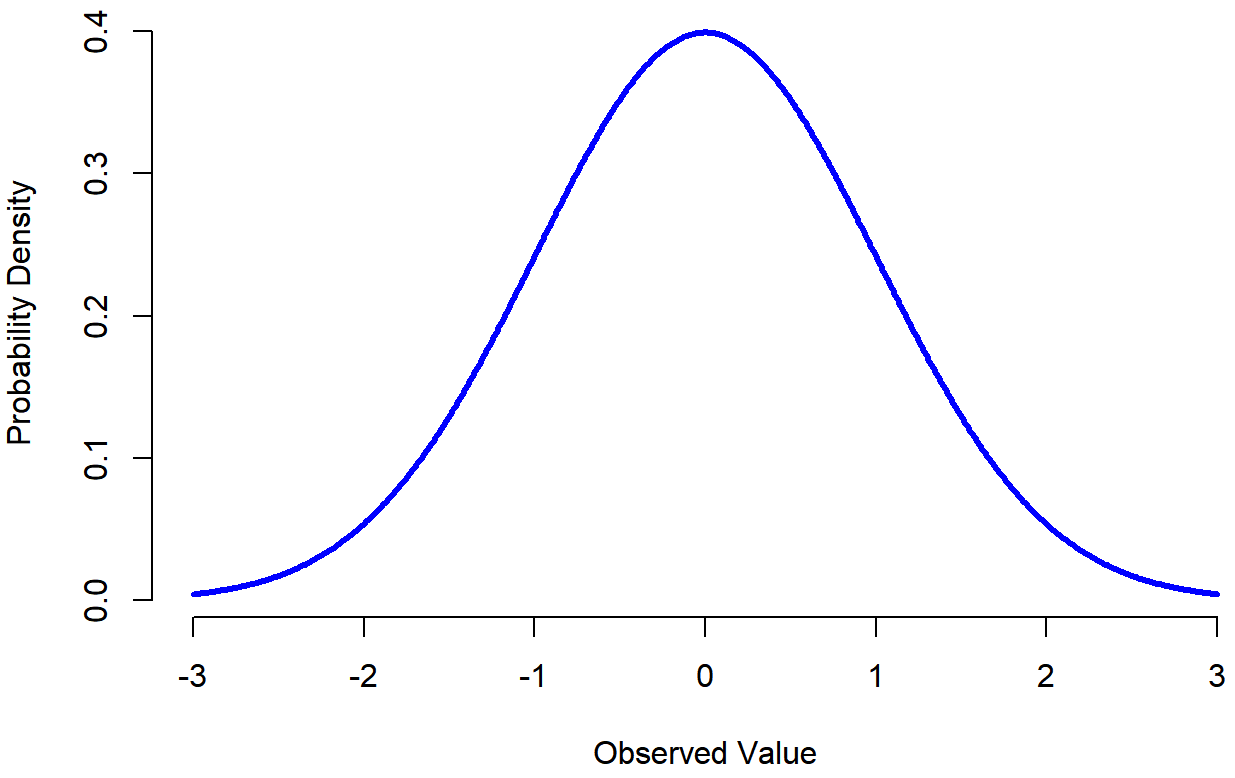
You can see where the name “bell curve” comes from in Figure \(\PageIndex{1}\) it looks a bit like a bell. Notice that, unlike the plots that I drew to illustrate the binomial distribution, the picture of the normal distribution in Figure \(\PageIndex{1}\) shows a smooth curve instead of “histogram-like” bars. This isn’t an arbitrary choice: the normal distribution is continuous, whereas the binomial is discrete. For instance, in the die rolling example, it was possible to get 3 skulls or 4 skulls, but impossible to get 3.9 skulls. The figures that I drew in the previous section reflected this fact. Continuous quantities don’t have this constraint. For instance, suppose we’re talking about the weather. The temperature on a pleasant Spring day could be 23 degrees, 24 degrees, 23.9 degrees, or anything in between since temperature is a continuous variable, and so a normal distribution might be quite appropriate for describing Spring temperatures.
- Normal Distributions: I know that there are predictable portions of scores between the mean and standard deviation.
The last important piece is learning that a special feature of normal distributions is that we know the proportions (percentages) of cases that should (probability) fall within each standard deviation around the mean. Irrespective of what the actual mean and standard deviation are, 68.3% of the area falls within 1 standard deviation of the mean. Similarly, 95.4% of the distribution falls within 2 standard deviations of the mean, and 99.7% of the distribution is within 3 standard deviations. This idea is illustrated in the follow Figures.
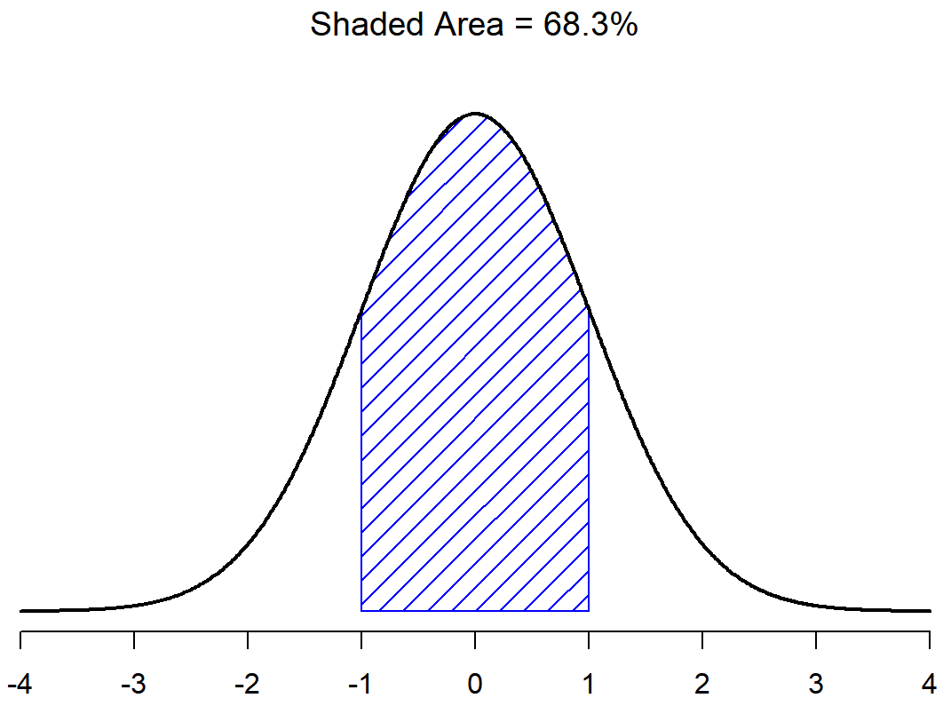
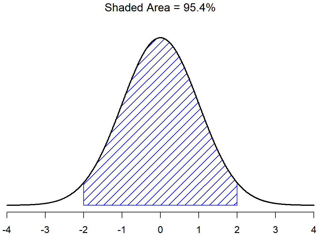
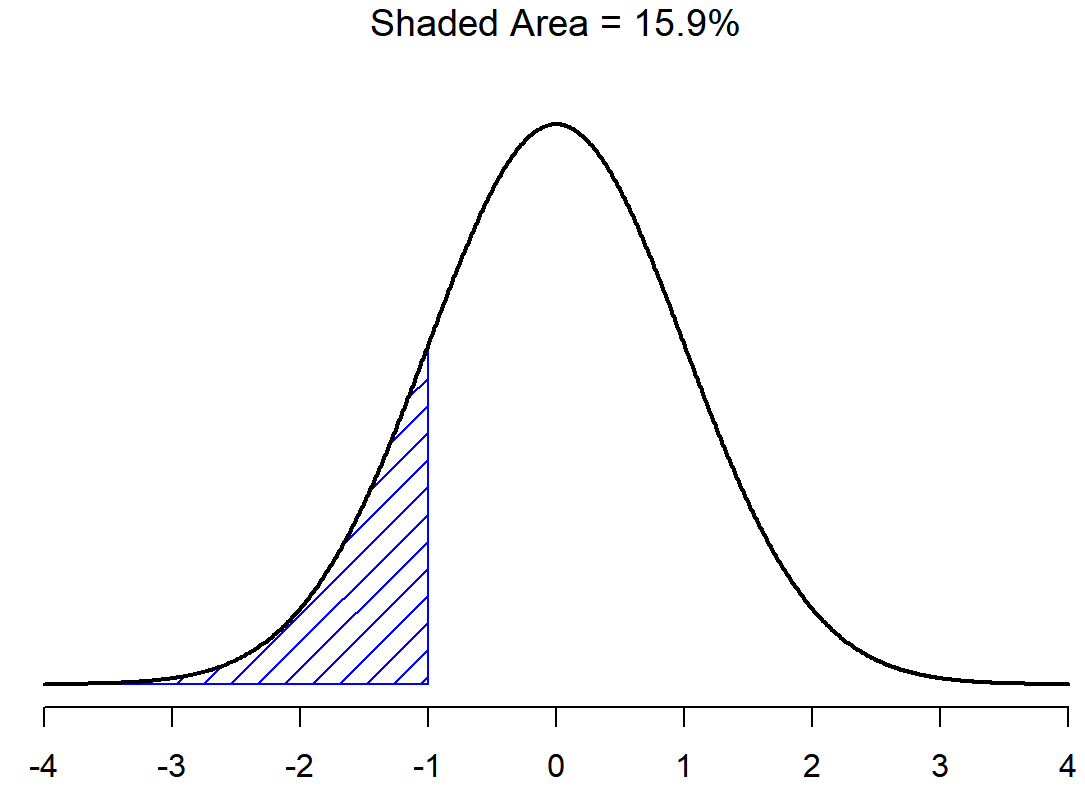
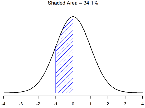
There is a 68.3% chance that a score from any sample will fall within the shaded area of Figure \(\PageIndex{2}\), and a 95.4% chance that an observation will fall within two standard deviations of the mean (the shaded area in Figure \(\PageIndex{3}\)). Similarly, there is a 15.9% chance that an observation will be below one standard deviation below the mean. There is a 34.1% chance that the observation is greater than one standard deviation below the mean but still below the mean (Figure \(\PageIndex{5}\)). Notice that if you add these two numbers together you get 15.9+34.1=50. For normally distributed data, there is a 50% chance that an observation falls below the mean. And of course that also implies that there is a 50% chance that it falls above the mean.
Continuous Variables
There’s something Dr. Navarro was trying to hide throughout this discussion of the normal distribution, but she just couldn't do it. Many introductory textbooks omit this completely; they might be right to do so: this “thing” that I’m hiding is weird and counterintuitive even by the admittedly distorted standards that apply in statistics. Fortunately, it’s not something that you need to understand at a deep level in order to do basic statistics: rather, it’s something that starts to become important later on when you move beyond the basics. So, if it doesn’t make complete sense, don’t worry: I'm mostly going over it to help think about the differences between qualitative and quantitative variables, and how quantitative variables can be discrete or continuous (even though we act like they are continuous).
Throughout the discussion of the normal distribution, there’s been one or two things that don’t quite make sense. Perhaps you noticed that the y-axis in these figures is labeled “Probability Density” rather than density. Let's spend a little time thinking about what it really means to say that X is a continuous variable. Let’s say we’re talking about the temperature outside. The thermometer tells me it’s 23 degrees, but I know that’s not really true. It’s not exactly 23 degrees. Maybe it’s 23.1 degrees, I think to myself. But I know that that’s not really true either, because it might actually be 23.09 degrees. But, I know that… well, you get the idea. The tricky thing with genuinely continuous quantities is that you never really know exactly what they are.
Now think about what this implies when we talk about probabilities. Suppose that tomorrow’s maximum temperature is sampled from a normal distribution with mean 23 and standard deviation 1. What’s the probability that the temperature will be exactly 23 degrees? The answer is “zero”, or possibly, “a number so close to zero that it might as well be zero”. Why is this? It’s like trying to throw a dart at an infinitely small dart board: no matter how good your aim, you’ll never hit it. In real life you’ll never get a value of exactly 23. It’ll always be something like 23.1 or 22.99998 or something. In other words, it’s completely meaningless to talk about the probability that the temperature is exactly 23 degrees. However, in everyday language, if I told you that it was 23 degrees outside and it turned out to be 22.9998 degrees, you probably wouldn’t call me a liar. Because in everyday language, “23 degrees” usually means something like “somewhere between 22.5 and 23.5 degrees”. And while it doesn’t feel very meaningful to ask about the probability that the temperature is exactly 23 degrees, it does seem sensible to ask about the probability that the temperature lies between 22.5 and 23.5, or between 20 and 30, or any other range of temperatures.
The point of this discussion is to make clear that, when we’re talking about continuous distributions, it’s not meaningful to talk about the probability of a specific value. However, what we can talk about is the probability that the value lies within a particular range of values. To find out the probability associated with a particular range, what you need to do is calculate the “area under the curve”. We’ve seen this concept already: in Figure \(\PageIndex{2}\), the shaded areas shown depict genuine probabilities (e.g., in Figure \(\PageIndex{2}\) it shows the probability of observing a value that falls within 1 standard deviation of the mean).
Okay, so that explains part of the story. I’ve explained a little bit about how continuous probability distributions should be interpreted (i.e., area under the curve is the key thing). In terms of the plots we’ve been drawing, probability density corresponds to the height of the curve. The densities themselves aren’t meaningful in and of themselves: but they’re “rigged” to ensure that the area under the curve is always interpretable as genuine probabilities. To be honest, that’s about as much as you really need to know for now.
We are about to finish up learning abstract theory about distributions, and moving on to actually using them!


