13.5: Anxiety and Depression

Anxiety and depression are often reported to be highly linked (or “comorbid”). Our hypothesis testing procedure follows the same four-step process as before, starting with our null and alternative hypotheses. We will look for a positive relation between our variables among a group of 10 people because that is what we would expect based on them being comorbid.

Step 1: State the Hypotheses

Our hypotheses for correlations start with a baseline assumption of no relation, and our alternative will be directional if we expect to find a specific type of relation. For this example, we expect a positive relation:

\[\begin{array}{c}{\mathrm{H}_{0}: \text { There is no positive relation between anxiety and depression}} \\ {\mathrm{H}_{0}: \rho \leq 0}\end{array} \nonumber \]

\[\begin{array}{c}{\mathrm{H}_{\mathrm{A}}: \text {There is a positive relation between anxiety and depression}} \\ {\mathrm{H}_{0}: \rho>0}\end{array} \nonumber \]

Remember that \(ρ\) (“rho”) is our population parameter for the correlation that we estimate with \(r\), just like \(M\) and \(μ\) for means. Remember also that if there is no relation between variables, the magnitude will be 0, which is where we get the null and alternative hypothesis values.

Step 2: Find the Critical Values

The critical values for correlations come from the correlation table, which looks very similar to the \(t\)-table (see Figure \(\PageIndex{1}\)). Just like our \(t\)-table, the column of critical values is based on our significance level (\(α\)) and the directionality of our test. The row is determined by our degrees of freedom. For correlations, we have \(N – 2\) degrees of freedom, rather than \(N – 1\) (why this is the case is not important). For our example, we have 10 people, so our degrees of freedom = 10 – 2 = 8.

Figure \(\PageIndex{1}\): Correlation table

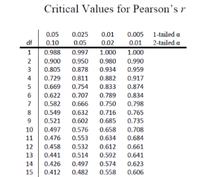
We were not given any information about the level of significance at which we should test our hypothesis, so we will assume \(α = 0.05\) as always. From our table, we can see that a 1-tailed test (because we expect only a positive relation) at the \(α = 0.05\) level has a critical value of \(r^* = 0.549\). Thus, if our observed correlation is greater than 0.549, it will be statistically significant. This is a rather high bar (remember, the guideline for a strong relation is \(r\) = 0.50); this is because we have so few people. Larger samples make it easier to find significant relations.

Step 3: Calculate the Test Statistic

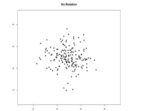
We have laid out our hypotheses and the criteria we will use to assess them, so now we can move on to our test statistic. Before we do that, we must first create a scatterplot of the data to make sure that the most likely form of our relation is in fact linear. Figure \(\PageIndex{2}\) below shows our data plotted out, and it looks like they are, in fact, linearly related, so Pearson’s \(r\) is appropriate.

Figure \(\PageIndex{2}\): Scatterplot of anxiety and depression

The data we gather from our participants is as follows:

Table \(\PageIndex{1}\): Data from participants

Dep	2.81	1.96	3.43	3.40	4.71	1.80	4.27	3.68	2.44	3.13
Anx	3.54	3.05	3.81	3.43	4.03	3.59	4.17	3.46	3.19	4.12

We will need to put these values into our Sum of Products table to calculate the standard deviation and covariance of our variables. We will use \(X\) for depression and \(Y\) for anxiety to keep track of our data, but be aware that this choice is arbitrary and the math will work out the same if we decided to do the opposite. Our table is thus:

Table \(\PageIndex{2}\): Sum of Products table

\(X\)	\((X-M_X)\)	\((X-M_X)^2\)	\(Y\)	\((Y-M _Y)\)	\((Y-M_Y)^2\)	\((X-M_X)(Y-M_Y)\)
2.81	-0.35	0.12	3.54	-0.10	0.01	0.04
1.96	-1.20	1.44	3.05	-0.59	0.35	0.71
3.43	0.27	0.07	3.81	0.17	0.03	0.05
3.40	0.24	0.06	3.43	-0.21	0.04	-0.05
4.71	1.55	2.40	4.03	0.39	0.15	0.60
1.80	-1.36	1.85	3.59	-0.05	0.00	0.07
4.27	1.11	1.23	4.17	0.53	0.28	0.59
3.68	0.52	0.27	3.46	-0.18	0.03	-0.09
2.44	-0.72	0.52	3.19	-0.45	0.20	0.32
3.13	-0.03	0.00	4.12	0.48	0.23	-0.01
31.63	0.03	7.97	36.39	-0.01	1.33	2.22

The bottom row is the sum of each column. We can see from this that the sum of the \(X\) observations is 31.63, which makes the mean of the \(X\) variable \(M_X=3.16\). The deviation scores for \(X\) sum to 0.03, which is very close to 0, given rounding error, so everything looks right so far. The next column is the squared deviations for \(X\), so we can see that the sum of squares for \(X\) is \(SS_X = 7.97\). The same is true of the \(Y\) columns, with an average of \(M_Y = 3.64\), deviations that sum to zero within rounding error, and a sum of squares as \(SS_Y = 1.33\). The final column is the product of our deviation scores (NOT of our squared deviations), which gives us a sum of products of \(SP = 2.22\).

There are now three pieces of information we need to calculate before we compute our correlation coefficient: the covariance of \(X\) and \(Y\) and the standard deviation of each.

The covariance of two variable, remember, is the sum of products divided by \(N – 1\). For our data:

\[\operatorname{cov}_{X Y}=\dfrac{S P}{N-1}=\dfrac{2.22}{9}=0.25 \nonumber \]

The formula for standard deviation are the same as before. Using subscripts \(X\) and \(Y\) to denote depression and anxiety:

\[s_{X}=\sqrt{\dfrac{\sum(X-M_X)^{2}}{N-1}}=\sqrt{\dfrac{7.97}{9}}=0.94 \nonumber \]

\[s_{Y}=\sqrt{\dfrac{\sum(Y-M_Y)^{2}}{N-1}}=\sqrt{\dfrac{1.33}{9}}=0.38 \nonumber \]

Now we have all of the information we need to calculate \(r\):

\[r=\dfrac{\operatorname{cov}_{X Y}}{s_{X} s_{Y}}=\dfrac{0.25}{0.94 * 0.38}=0.70 \nonumber \]

We can verify this using our other formula, which is computationally shorter:

\[r=\dfrac{S P}{\sqrt{SS_X * SS_Y}}=\dfrac{2.22}{\sqrt{7.97 * 1.33}}=.70 \nonumber \]

So our observed correlation between anxiety and depression is \(r = 0.70\), which, based on sign and magnitude, is a strong, positive correlation. Now we need to compare it to our critical value to see if it is also statistically significant.

Step 4: Make a Decision

Our critical value was \(r^* = 0.549\) and our obtained value was \(r = 0.70\). Our obtained value was larger than our critical value, so we can reject the null hypothesis.

Reject \(H_0\). Based on our sample of 10 people, there is a statistically significant, strong, positive relation between anxiety and depression, \(r(8) = 0.70, p < .05\).

Notice in our interpretation that, because we already know the magnitude and direction of our correlation, we can interpret that. We also report the degrees of freedom, just like with \(t\), and we know that \(p < α\) because we rejected the null hypothesis. As we can see, even though we are dealing with a very different type of data, our process of hypothesis testing has remained unchanged.

Contributors and Attributions

• Foster et al. (University of Missouri-St. Louis, Rice University, & University of Houston, Downtown Campus)