Learning Objectives
- For a linear relationship, use the least squares regression line to model the pattern in the data and to make predictions.
Let’s quickly revisit the list of our data analysis tools for working with linear relationships:
- Use a scatterplot and r to describe direction and strength of the linear relationship.
- Find the equation of the least-squares regression line to summarize the relationship.
- Use the equation and the graph of the least-squares line to make predictions.
- Avoid extrapolation when making predictions.
Now we focus on the equation of a line in more detail. Our goal is to understand what the numbers in the equation tell us about the relationship between the explanatory variable and the response variable.
Here are some of the equations of lines that we have used in our discussion of linear relationships:
Predicted distance = 576 − 3 * Age
Predicted height = 39 + 2.7 * forearm length
Predicted monthly car insurance premium = 97 − 1.45 * years of driving experience
Notice that the form of the equations is the same. In general, each equation has the form
Predicted y = a + b * x
When we find the least-squares regression line, a and b are determined by the data. The values of a and b do not change, so we refer to them as constants.
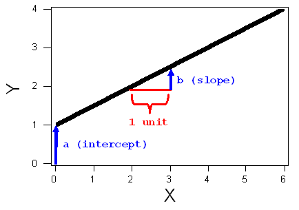
In the equation of the line, the constant a is the prediction when x = 0. It is called initial value. In a graph of the line, a is the y-intercept.
In the equation of the line, the constant b is the rate of change, called the slope. In a graph of the least-squares line, b describes how the predictions change when x increases by one unit. More specifically, b describes the average change in the response variable when the explanatory variable increases by one unit.
We can write the equation of the line to reflect the meaning of a and b:
Predicted y = a + b * x
Predicted y-value = (initial value) + (rate of change)*x
Predicted y-value = (y-intercept) + (slope)*x
The constants a and b are shown in the graph of the line below.

Algebra review
The algebra of a line
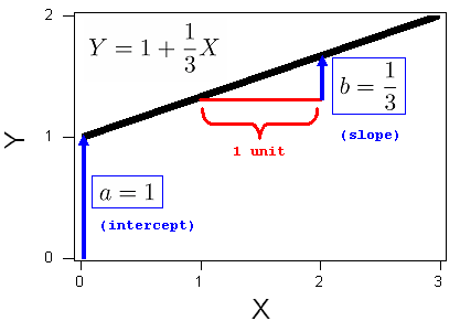
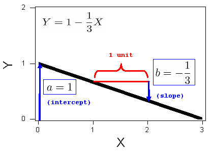
The general form for the equation of a line is Y = a + bX. The constants “a” and “b” can be either positive or negative. The constant “a” is the y-intercept where the line crosses the y-axis. The constant “b” is the slope. It describes the steepness of the line. In algebra we describe the slope as “rise over run”. The slope is the amount that Y increases (or decreases) for each 1-unit increase in X.
EXAMPLE
1
Consider the line  . The intercept is 1. The slope is 1/3, and the graph of this line is, therefore:
EXAMPLE
2
Consider the line  . The intercept is 1. The slope is -1/3, and the graph of this line is, therefore:
The simulation below allows you to see how changing the values of the slope and y-intercept changes the line. The slider on the left controls the y-intercept, a. The slider on the right controls the slope, b.
Use the simulation to draw the following lines:
Y = 3 + 0.67X
Y = 5 – X (which can also be written Y = 5 – 1.0X)
Y = 2X (which can also be written Y = 0 + 2X)
Y = 5 – 2X
A link to an interactive elements can be found at the bottom of this page.
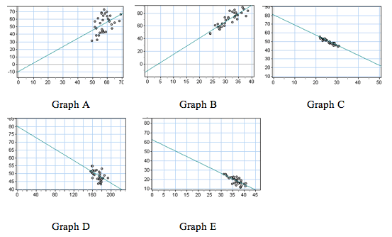
Use the following graphs in the next activity to investigate the equation of lines.

Interpreting the Slope and Intercept
The constants in the equation of a line give us important information about the relationship between the predictions and x. In the next examples, we focus on how to interpret the meaning of the constants in the context of data.
Example
Highway Sign Visibility Data
Recall that from a data set of 30 drivers, we see a strong negative linear relationship between the age of a driver (x) and the maximum distance (in feet) at which a driver can read a highway sign. The least-squares regression line is
Predicted y-value = (starting value) + (rate of change)*x
Predicted distance = 576 − 3 * Age
Predicted distance = 576 + (−3 * Age)
The value of b is −3. This means that a 1-year increase in age corresponds to a predicted 3-foot decrease in maximum distance at which a driver can read a sign. Another way to say this is that there is an average decrease of 3 feet in predicted sign visibility distance when we compare drivers of age x to drivers of age x + 1.
The 576 is the predicted value when x = 0. Obviously, it does not make sense to predict a maximum sign visibility distance for a driver who is 0 years old. This is an example of extrapolating outside the range of the data. But the starting value is an important part of the least-squares equation for predicting distances based on age.
The equation tells us that to predict the maximum visibility distance for a driver, start with a distance of 576 feet and subtract 3 feet for every year of the driver’s age.
Example
Body Measurements
In the body measurement data collected from 21 female community college students, we found a strong positive correlation between forearm length and height. The least-squares regression line is
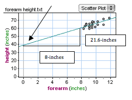
Predicted height = 39 + 2.7 * forearm length
The value of b is 2.7. This means that a 1-inch increase in forearm length corresponds to a predicted 2.7-inch increase in height. Another way to say this is that there is an average increase of 2.7-inches in predicted height when we compare women with forearm length of x to women with forearm length of x + 1.
The 39 is the predicted value when x = 0. Obviously, it does not make sense to predict the height of a woman with a 0-inch forearm length. This is another example of extrapolating outside the range of the data. But 39 inches is the starting value in the least-squares equation for predicting height based on forearm length.
The equation tells us that to predict the height of a woman, start with 39 inches and add 2.7 inches for every inch of forearm length.
In the graph below, we see the slope b represented by a triangle. An 8-inch increase in foreman length corresponds to a 21.6-inch increase in predicted height. b = 21.6 / 8 = 2.7. An arrow points to the starting value a = 39. This is the point with x = 0.

Contributors and Attributions
CC licensed content, Shared previously


