
6.4: One- and Two-Tailed Tests
- Page ID
- 28910

\( \newcommand{\vecs}[1]{\overset { \scriptstyle \rightharpoonup} {\mathbf{#1}} } \)
\( \newcommand{\vecd}[1]{\overset{-\!-\!\rightharpoonup}{\vphantom{a}\smash {#1}}} \)
\( \newcommand{\dsum}{\displaystyle\sum\limits} \)
\( \newcommand{\dint}{\displaystyle\int\limits} \)
\( \newcommand{\dlim}{\displaystyle\lim\limits} \)
\( \newcommand{\id}{\mathrm{id}}\) \( \newcommand{\Span}{\mathrm{span}}\)
( \newcommand{\kernel}{\mathrm{null}\,}\) \( \newcommand{\range}{\mathrm{range}\,}\)
\( \newcommand{\RealPart}{\mathrm{Re}}\) \( \newcommand{\ImaginaryPart}{\mathrm{Im}}\)
\( \newcommand{\Argument}{\mathrm{Arg}}\) \( \newcommand{\norm}[1]{\| #1 \|}\)
\( \newcommand{\inner}[2]{\langle #1, #2 \rangle}\)
\( \newcommand{\Span}{\mathrm{span}}\)
\( \newcommand{\id}{\mathrm{id}}\)
\( \newcommand{\Span}{\mathrm{span}}\)
\( \newcommand{\kernel}{\mathrm{null}\,}\)
\( \newcommand{\range}{\mathrm{range}\,}\)
\( \newcommand{\RealPart}{\mathrm{Re}}\)
\( \newcommand{\ImaginaryPart}{\mathrm{Im}}\)
\( \newcommand{\Argument}{\mathrm{Arg}}\)
\( \newcommand{\norm}[1]{\| #1 \|}\)
\( \newcommand{\inner}[2]{\langle #1, #2 \rangle}\)
\( \newcommand{\Span}{\mathrm{span}}\) \( \newcommand{\AA}{\unicode[.8,0]{x212B}}\)
\( \newcommand{\vectorA}[1]{\vec{#1}} % arrow\)
\( \newcommand{\vectorAt}[1]{\vec{\text{#1}}} % arrow\)
\( \newcommand{\vectorB}[1]{\overset { \scriptstyle \rightharpoonup} {\mathbf{#1}} } \)
\( \newcommand{\vectorC}[1]{\textbf{#1}} \)
\( \newcommand{\vectorD}[1]{\overrightarrow{#1}} \)
\( \newcommand{\vectorDt}[1]{\overrightarrow{\text{#1}}} \)
\( \newcommand{\vectE}[1]{\overset{-\!-\!\rightharpoonup}{\vphantom{a}\smash{\mathbf {#1}}}} \)
\( \newcommand{\vecs}[1]{\overset { \scriptstyle \rightharpoonup} {\mathbf{#1}} } \)
\(\newcommand{\longvect}{\overrightarrow}\)
\( \newcommand{\vecd}[1]{\overset{-\!-\!\rightharpoonup}{\vphantom{a}\smash {#1}}} \)
\(\newcommand{\avec}{\mathbf a}\) \(\newcommand{\bvec}{\mathbf b}\) \(\newcommand{\cvec}{\mathbf c}\) \(\newcommand{\dvec}{\mathbf d}\) \(\newcommand{\dtil}{\widetilde{\mathbf d}}\) \(\newcommand{\evec}{\mathbf e}\) \(\newcommand{\fvec}{\mathbf f}\) \(\newcommand{\nvec}{\mathbf n}\) \(\newcommand{\pvec}{\mathbf p}\) \(\newcommand{\qvec}{\mathbf q}\) \(\newcommand{\svec}{\mathbf s}\) \(\newcommand{\tvec}{\mathbf t}\) \(\newcommand{\uvec}{\mathbf u}\) \(\newcommand{\vvec}{\mathbf v}\) \(\newcommand{\wvec}{\mathbf w}\) \(\newcommand{\xvec}{\mathbf x}\) \(\newcommand{\yvec}{\mathbf y}\) \(\newcommand{\zvec}{\mathbf z}\) \(\newcommand{\rvec}{\mathbf r}\) \(\newcommand{\mvec}{\mathbf m}\) \(\newcommand{\zerovec}{\mathbf 0}\) \(\newcommand{\onevec}{\mathbf 1}\) \(\newcommand{\real}{\mathbb R}\) \(\newcommand{\twovec}[2]{\left[\begin{array}{r}#1 \\ #2 \end{array}\right]}\) \(\newcommand{\ctwovec}[2]{\left[\begin{array}{c}#1 \\ #2 \end{array}\right]}\) \(\newcommand{\threevec}[3]{\left[\begin{array}{r}#1 \\ #2 \\ #3 \end{array}\right]}\) \(\newcommand{\cthreevec}[3]{\left[\begin{array}{c}#1 \\ #2 \\ #3 \end{array}\right]}\) \(\newcommand{\fourvec}[4]{\left[\begin{array}{r}#1 \\ #2 \\ #3 \\ #4 \end{array}\right]}\) \(\newcommand{\cfourvec}[4]{\left[\begin{array}{c}#1 \\ #2 \\ #3 \\ #4 \end{array}\right]}\) \(\newcommand{\fivevec}[5]{\left[\begin{array}{r}#1 \\ #2 \\ #3 \\ #4 \\ #5 \\ \end{array}\right]}\) \(\newcommand{\cfivevec}[5]{\left[\begin{array}{c}#1 \\ #2 \\ #3 \\ #4 \\ #5 \\ \end{array}\right]}\) \(\newcommand{\mattwo}[4]{\left[\begin{array}{rr}#1 \amp #2 \\ #3 \amp #4 \\ \end{array}\right]}\) \(\newcommand{\laspan}[1]{\text{Span}\{#1\}}\) \(\newcommand{\bcal}{\cal B}\) \(\newcommand{\ccal}{\cal C}\) \(\newcommand{\scal}{\cal S}\) \(\newcommand{\wcal}{\cal W}\) \(\newcommand{\ecal}{\cal E}\) \(\newcommand{\coords}[2]{\left\{#1\right\}_{#2}}\) \(\newcommand{\gray}[1]{\color{gray}{#1}}\) \(\newcommand{\lgray}[1]{\color{lightgray}{#1}}\) \(\newcommand{\rank}{\operatorname{rank}}\) \(\newcommand{\row}{\text{Row}}\) \(\newcommand{\col}{\text{Col}}\) \(\renewcommand{\row}{\text{Row}}\) \(\newcommand{\nul}{\text{Nul}}\) \(\newcommand{\var}{\text{Var}}\) \(\newcommand{\corr}{\text{corr}}\) \(\newcommand{\len}[1]{\left|#1\right|}\) \(\newcommand{\bbar}{\overline{\bvec}}\) \(\newcommand{\bhat}{\widehat{\bvec}}\) \(\newcommand{\bperp}{\bvec^\perp}\) \(\newcommand{\xhat}{\widehat{\xvec}}\) \(\newcommand{\vhat}{\widehat{\vvec}}\) \(\newcommand{\uhat}{\widehat{\uvec}}\) \(\newcommand{\what}{\widehat{\wvec}}\) \(\newcommand{\Sighat}{\widehat{\Sigma}}\) \(\newcommand{\lt}{<}\) \(\newcommand{\gt}{>}\) \(\newcommand{\amp}{&}\) \(\definecolor{fillinmathshade}{gray}{0.9}\)Learning Objectives
- Define Type I and Type II errors
- Interpret significant and non-significant differences
- Explain why the null hypothesis should not be accepted when the effect is not significant
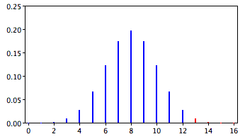
In the James Bond case study, Mr. Bond was given \(16\) trials on which he judged whether a martini had been shaken or stirred. He was correct on \(13\) of the trials. From the binomial distribution, we know that the probability of being correct \(13\) or more times out of \(16\) if one is only guessing is \(0.0106\). Figure \(\PageIndex{1}\) shows a graph of the binomial distribution. The red bars show the values greater than or equal to \(13\). As you can see in the figure, the probabilities are calculated for the upper tail of the distribution. A probability calculated in only one tail of the distribution is called a "one-tailed probability."
Binomial Calculator
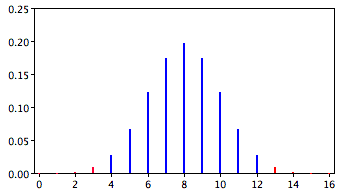
A slightly different question can be asked of the data: "What is the probability of getting a result as extreme or more extreme than the one observed?" Since the chance expectation is \(8/16\), a result of \(3/16\) is equally as extreme as \(13/16\). Thus, to calculate this probability, we would consider both tails of the distribution. Since the binomial distribution is symmetric when \(\pi =0.5\), this probability is exactly double the probability of \(0.0106\) computed previously. Therefore, \(p = 0.0212\). A probability calculated in both tails of a distribution is called a "two-tailed probability" (see Figure \(\PageIndex{2}\)).
Should the one-tailed or the two-tailed probability be used to assess Mr. Bond's performance? That depends on the way the question is posed. If we are asking whether Mr. Bond can tell the difference between shaken or stirred martinis, then we would conclude he could if he performed either much better than chance or much worse than chance. If he performed much worse than chance, we would conclude that he can tell the difference, but he does not know which is which. Therefore, since we are going to reject the null hypothesis if Mr. Bond does either very well or very poorly, we will use a two-tailed probability.
On the other hand, if our question is whether Mr. Bond is better than chance at determining whether a martini is shaken or stirred, we would use a one-tailed probability. What would the one-tailed probability be if Mr. Bond were correct on only \(3\) of the \(16\) trials? Since the one-tailed probability is the probability of the right-hand tail, it would be the probability of getting \(3\) or more correct out of \(16\). This is a very high probability and the null hypothesis would not be rejected.
The null hypothesis for the two-tailed test is \(\pi =0.5\). By contrast, the null hypothesis for the one-tailed test is \(\pi \leq 0.5\). Accordingly, we reject the two-tailed hypothesis if the sample proportion deviates greatly from \(0.5\) in either direction. The one-tailed hypothesis is rejected only if the sample proportion is much greater than \(0.5\). The alternative hypothesis in the two-tailed test is \(\pi \neq 0.5\). In the one-tailed test it is \(\pi > 0.5\).
You should always decide whether you are going to use a one-tailed or a two-tailed probability before looking at the data. Statistical tests that compute one-tailed probabilities are called one-tailed tests; those that compute two-tailed probabilities are called two-tailed tests. Two-tailed tests are much more common than one-tailed tests in scientific research because an outcome signifying that something other than chance is operating is usually worth noting. One-tailed tests are appropriate when it is not important to distinguish between no effect and an effect in the unexpected direction. For example, consider an experiment designed to test the efficacy of a treatment for the common cold. The researcher would only be interested in whether the treatment was better than a placebo control. It would not be worth distinguishing between the case in which the treatment was worse than a placebo and the case in which it was the same because in both cases the drug would be worthless.
Some have argued that a one-tailed test is justified whenever the researcher predicts the direction of an effect. The problem with this argument is that if the effect comes out strongly in the non-predicted direction, the researcher is not justified in concluding that the effect is not zero. Since this is unrealistic, one-tailed tests are usually viewed skeptically if justified on this basis alone.