6.2: Using the Normal Distribution
- Page ID
- 16256
\( \newcommand{\vecs}[1]{\overset { \scriptstyle \rightharpoonup} {\mathbf{#1}} } \)
\( \newcommand{\vecd}[1]{\overset{-\!-\!\rightharpoonup}{\vphantom{a}\smash {#1}}} \)
\( \newcommand{\id}{\mathrm{id}}\) \( \newcommand{\Span}{\mathrm{span}}\)
( \newcommand{\kernel}{\mathrm{null}\,}\) \( \newcommand{\range}{\mathrm{range}\,}\)
\( \newcommand{\RealPart}{\mathrm{Re}}\) \( \newcommand{\ImaginaryPart}{\mathrm{Im}}\)
\( \newcommand{\Argument}{\mathrm{Arg}}\) \( \newcommand{\norm}[1]{\| #1 \|}\)
\( \newcommand{\inner}[2]{\langle #1, #2 \rangle}\)
\( \newcommand{\Span}{\mathrm{span}}\)
\( \newcommand{\id}{\mathrm{id}}\)
\( \newcommand{\Span}{\mathrm{span}}\)
\( \newcommand{\kernel}{\mathrm{null}\,}\)
\( \newcommand{\range}{\mathrm{range}\,}\)
\( \newcommand{\RealPart}{\mathrm{Re}}\)
\( \newcommand{\ImaginaryPart}{\mathrm{Im}}\)
\( \newcommand{\Argument}{\mathrm{Arg}}\)
\( \newcommand{\norm}[1]{\| #1 \|}\)
\( \newcommand{\inner}[2]{\langle #1, #2 \rangle}\)
\( \newcommand{\Span}{\mathrm{span}}\) \( \newcommand{\AA}{\unicode[.8,0]{x212B}}\)
\( \newcommand{\vectorA}[1]{\vec{#1}} % arrow\)
\( \newcommand{\vectorAt}[1]{\vec{\text{#1}}} % arrow\)
\( \newcommand{\vectorB}[1]{\overset { \scriptstyle \rightharpoonup} {\mathbf{#1}} } \)
\( \newcommand{\vectorC}[1]{\textbf{#1}} \)
\( \newcommand{\vectorD}[1]{\overrightarrow{#1}} \)
\( \newcommand{\vectorDt}[1]{\overrightarrow{\text{#1}}} \)
\( \newcommand{\vectE}[1]{\overset{-\!-\!\rightharpoonup}{\vphantom{a}\smash{\mathbf {#1}}}} \)
\( \newcommand{\vecs}[1]{\overset { \scriptstyle \rightharpoonup} {\mathbf{#1}} } \)
\( \newcommand{\vecd}[1]{\overset{-\!-\!\rightharpoonup}{\vphantom{a}\smash {#1}}} \)
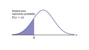
\(\newcommand{\avec}{\mathbf a}\) \(\newcommand{\bvec}{\mathbf b}\) \(\newcommand{\cvec}{\mathbf c}\) \(\newcommand{\dvec}{\mathbf d}\) \(\newcommand{\dtil}{\widetilde{\mathbf d}}\) \(\newcommand{\evec}{\mathbf e}\) \(\newcommand{\fvec}{\mathbf f}\) \(\newcommand{\nvec}{\mathbf n}\) \(\newcommand{\pvec}{\mathbf p}\) \(\newcommand{\qvec}{\mathbf q}\) \(\newcommand{\svec}{\mathbf s}\) \(\newcommand{\tvec}{\mathbf t}\) \(\newcommand{\uvec}{\mathbf u}\) \(\newcommand{\vvec}{\mathbf v}\) \(\newcommand{\wvec}{\mathbf w}\) \(\newcommand{\xvec}{\mathbf x}\) \(\newcommand{\yvec}{\mathbf y}\) \(\newcommand{\zvec}{\mathbf z}\) \(\newcommand{\rvec}{\mathbf r}\) \(\newcommand{\mvec}{\mathbf m}\) \(\newcommand{\zerovec}{\mathbf 0}\) \(\newcommand{\onevec}{\mathbf 1}\) \(\newcommand{\real}{\mathbb R}\) \(\newcommand{\twovec}[2]{\left[\begin{array}{r}#1 \\ #2 \end{array}\right]}\) \(\newcommand{\ctwovec}[2]{\left[\begin{array}{c}#1 \\ #2 \end{array}\right]}\) \(\newcommand{\threevec}[3]{\left[\begin{array}{r}#1 \\ #2 \\ #3 \end{array}\right]}\) \(\newcommand{\cthreevec}[3]{\left[\begin{array}{c}#1 \\ #2 \\ #3 \end{array}\right]}\) \(\newcommand{\fourvec}[4]{\left[\begin{array}{r}#1 \\ #2 \\ #3 \\ #4 \end{array}\right]}\) \(\newcommand{\cfourvec}[4]{\left[\begin{array}{c}#1 \\ #2 \\ #3 \\ #4 \end{array}\right]}\) \(\newcommand{\fivevec}[5]{\left[\begin{array}{r}#1 \\ #2 \\ #3 \\ #4 \\ #5 \\ \end{array}\right]}\) \(\newcommand{\cfivevec}[5]{\left[\begin{array}{c}#1 \\ #2 \\ #3 \\ #4 \\ #5 \\ \end{array}\right]}\) \(\newcommand{\mattwo}[4]{\left[\begin{array}{rr}#1 \amp #2 \\ #3 \amp #4 \\ \end{array}\right]}\) \(\newcommand{\laspan}[1]{\text{Span}\{#1\}}\) \(\newcommand{\bcal}{\cal B}\) \(\newcommand{\ccal}{\cal C}\) \(\newcommand{\scal}{\cal S}\) \(\newcommand{\wcal}{\cal W}\) \(\newcommand{\ecal}{\cal E}\) \(\newcommand{\coords}[2]{\left\{#1\right\}_{#2}}\) \(\newcommand{\gray}[1]{\color{gray}{#1}}\) \(\newcommand{\lgray}[1]{\color{lightgray}{#1}}\) \(\newcommand{\rank}{\operatorname{rank}}\) \(\newcommand{\row}{\text{Row}}\) \(\newcommand{\col}{\text{Col}}\) \(\renewcommand{\row}{\text{Row}}\) \(\newcommand{\nul}{\text{Nul}}\) \(\newcommand{\var}{\text{Var}}\) \(\newcommand{\corr}{\text{corr}}\) \(\newcommand{\len}[1]{\left|#1\right|}\) \(\newcommand{\bbar}{\overline{\bvec}}\) \(\newcommand{\bhat}{\widehat{\bvec}}\) \(\newcommand{\bperp}{\bvec^\perp}\) \(\newcommand{\xhat}{\widehat{\xvec}}\) \(\newcommand{\vhat}{\widehat{\vvec}}\) \(\newcommand{\uhat}{\widehat{\uvec}}\) \(\newcommand{\what}{\widehat{\wvec}}\) \(\newcommand{\Sighat}{\widehat{\Sigma}}\) \(\newcommand{\lt}{<}\) \(\newcommand{\gt}{>}\) \(\newcommand{\amp}{&}\) \(\definecolor{fillinmathshade}{gray}{0.9}\) Theblue shaded area in the following graph indicates the area to the left of x.
P(X < a) = Area to the left of the vertical line through a. (blue area)
P(X > a) = Area to the right of the vertical line through a. (white area)
P(X > a) is also equal to 1 – P(X < a).
Remember,
P(X < a) = P(X ≤ a) and P(X > a) = P(X ≥ a) for continuous distributions.
Calculations of Probabilities
Probabilities are calculated using technology. There are instructions given as necessary for the TI-83+ and TI-84 calculators.
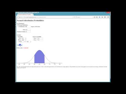
Additionally, this link houses a tool that allows you to explore the normal distribution with varying means and standard deviations as well as associated probabilities. The following video explains how to use the tool.
Example 1
If the area to the left is 0.0228, what is the area to the right?
[reveal-answer q=”885453″]Show Answer[/reveal-answer]
[hidden-answer a=”885453″]the area to the right is 1 – 0.0228 = 0.9772.[/hidden-answer]
Try It
If the area to the left of x is 0.012, then what is the area to the right?
[practice-area rows=”2″][/practice-area]
[reveal-answer q=”639208″]Show Answer[/reveal-answer]
[hidden-answer a=”639208″]1 − 0.012 = 0.988[/hidden-answer]
Example 2 (by using TI-83/84 Calculators)
The final exam scores in a statistics class were normally distributed with a mean of 63 and a standard deviation of 5.
- Find the probability that a randomly selected student scored more than 65 on the exam.
- Find the probability that a randomly selected student scored less than 85.
- Find the 90th percentile (that is, find the score k that has 90% of the scores below k and 10% of the scores above k).
- Find the 70th percentile (that is, find the score k such that 70% of scores are below k and 30% of the scores are above k).
Solution
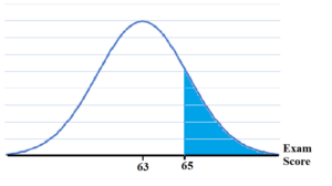
- Find the probability that a randomly selected student scored more than 65 on the exam.Let X = a score on the final exam. X ~ N(63, 5), where mean, μ = 63 and standard deviation,σ = 5.
- Draw a graph. Then, find P(x > 65).

- Using TI-Calculator:
Go into2nd DISTR. Then press2:normalcdf.
The syntax for the instructions are as follows: normalcdf (lower value, upper value, mean, standard deviation).
For this problem: normalcdf (65,10^99,63,5) and press “=”.
The answer is 0.3446. - Therefore, P(x > 65) = 0.3446.
The probability that any student selected at random scores more than 65 is 0.3446.
******************************************************************************************************************Extra Note:
The number 1099 is way out in the right tail of the normal curve. We are calculating the area when final exam score is between between 65 and 1099.
In some instances, the lower number of the area might be –1099.
The number –1099 is way out in the left tail of the normal curve.
We can solve that area to the left of z-score 0.4 is 0.6554 by inputting normalcdf(-10^99, 65, 63, 5) to TI-Calculator.
Hence, P(x > 65) = P(z > 0.4) = 1 – 0.6554 = 0.3446***************************************************************************************************************************
To calculate the z-score:
Press
2nd ---> Distr, and choose3:invNorm(*Enter the area to the left of z followed by ), and pressENTER.
For this Example, the steps are2nd ---> Distr --->3:invNorm(.6554) —>ENTER.The answer is 0.3999 which rounds to 0.4.
****************************************************************************************************************************
- Draw a graph. Then, find P(x > 65).
- Find the probability that a randomly selected student scored less than 85.Draw a graph to find P(x < 85), and shade the graph. Using a computer or calculator, find P(x < 85).[reveal-answer q=”133054″]Use calculator to try first before looking for the answer! [/reveal-answer]
[hidden-answer a=”133054″] TI-Calculator: normalcdf(-10^99,85,63,5). The answer is 1. (rounds to one)
The probability that one student scores less than 85 is approximately one (or 100%).[/hidden-answer] - Find the 90th percentile.For each problem or part of a problem, draw a new graph.
Draw the x-axis. Shade the area that corresponds to the 90th percentile.
Let k= the 90th percentile. The variable k is located on the x-axis. P(x < k) is the area to the left of k.
The 90th percentile k separates the exam scores into those that are the same or lower than k and those that are the same or higher. Ninety percent of the test scores are the same or lower than k, and ten percent are the same or higher.
The variable k is often called a critical value.
To get the answer on the calculator, follow this step: 2nd —> DISTR —>invNorm.
The format for this function is invNorm(area to the left, mean, standard deviation)
For this problem, we need to input “invNorm(0.90,63,5)” and press “=”.
The answer is 69.4.
So the 90th percentile is 69.4. This means that 90% of the test scores fall at or below 69.4 and 10% fall at or above. - Find the 70th percentile.Draw a new graph and label it appropriately. k = 65.6.[reveal-answer q=”184963″]Use calculator to try first before looking for the answer! [/reveal-answer]
[hidden-answer a=”184963″]invNorm(0.70,63,5) = 65.6[/hidden-answer]
The 70th percentile is 65.6.
This means that 70% of the test scores fall at or below 65.5 and 30% fall at or above.
Try It
The golf scores for a school team were normally distributed with a mean of 68 and a standard deviation of 3.
Find the probability that a randomly selected golfer scored less than 65.
[practice-area rows=”3″][/practice-area]
[reveal-answer q=”854393″]Show Answer[/reveal-answer]
[hidden-answer a=”854393″]
TI-Calculator: normalcdf(1099,65,68,3)
The proability that a randomly selected golfer scored less than 65 is 0.1587. [/hidden-answer]
Example 3
A personal computer is used for office work at home, research, communication, personal finances, education, entertainment, social networking, and a myriad of other things. Suppose that the average number of hours a household personal computer is used for entertainment is two hours per day. Assume the times for entertainment are normally distributed and the standard deviation for the times is half an hour.
- Find the probability that a household personal computer is used for entertainment between 1.8 and 2.75 hours per day.
- Find the maximum number of hours per day that the bottom quartile of households uses a personal computer for entertainment.
Solution
- Let X= the amount of time (in hours) a household personal computer is used for entertainment.
X ~ N(2, 0.5) where mean, μ = 2 and standard deviation, σ = 0.5.
Find P(1.8 < x < 2.75).The probability for which you are looking is the area betweenx = 1.8 and x = 2.75.
TI-Calculator: normalcdf(1.8,2.75,2,0.5). The answer is 0.5886.
P(1.8 < x < 2.75) = 0.5886.
The probability that a household personal computer is used between 1.8 and 2.75 hours per day for entertainment is 0.5886. - To find the maximum number of hours per day that the bottom quartile of households uses a personal computer for entertainment, we need to find the 25th percentile, k.
P(x < k) = 0.25.
TI-Calculator: invNorm(0.25,2,0.5) = 1.66.
The maximum number of hours per day that the bottom quartile of households uses a personal computer for entertainment is 1.66 hours.
Try It
The golf scores for a school team were normally distributed with a mean of 68 and a standard deviation of three. Find the probability that a golfer scored between 66 and 70.
[practice-area rows=”3″][/practice-area]
[reveal-answer q=”208977″]Show Answer[/reveal-answer]
[hidden-answer a=”208977″]
TI-Calculator: normalcdf(66,70,68,3)
The probability that a golfer scored between 66 and 70 is 0.4950[/hidden-answer]
Example 4
There are approximately one billion smartphone users in the world today. In the United States the ages 13 to 55+ of smartphone users approximately follow a normal distribution with approximate mean and standard deviation of 36.9 years and 13.9 years, respectively.
- Determine the probability that a random smartphone user in the age range 13 to 55+ is between 23 and 64.7 years old.
- Determine the probability that a randomly selected smartphone user in the age range 13 to 55+ is at most 50.8 years old.
- Find the 80th percentile of this distribution, and interpret it in a complete sentence.
Solution:
[reveal-answer q=”83966″]Show Answer[/reveal-answer]
[hidden-answer a=”83966″]
1. normalcdf(23,64.7,36.9,13.9) = 0.8186
2. normalcdf(–1099,50.8,36.9,13.9) = 0.8413
3. invNorm(0.80,36.9,13.9) = 48.6
The 80th percentile is 48.6 years.
80% of the smartphone users in the age range 13 – 55+ are 48.6 years old or less.[/hidden-answer]
Try It
Use the information in Example 3 to answer the following questions.
- Find the 30th percentile, and interpret it in a complete sentence.
- What is the probability that the age of a randomly selected smartphone user in the range 13 to 55+ is less than 27 years old.
Solution:
Let X = a smart phone user whose age is 13 to 55+. X ~ N(36.9, 13.9)
- To find the 30th percentile, find k such that P(x < k) = 0.30.
[reveal-answer q=”286436″]Show Answer[/reveal-answer]
[hidden-answer a=”286436″]
TI-Calculators: invNorm(0.30, 36.9, 13.9)
The solution is 29.6 years.
30% of smartphone users aged between 13 and 55+ are at most 29.6 years and 70% are at least 29.6 years.
[/hidden-answer] - Find P(x < 27).
[reveal-answer q=”266874″]Show Answer[/reveal-answer]
[hidden-answer a=”266874″]
TI-Calculators: invNorm(0.30, 36.9, 13.9)
The solution is 29.6 years.
30% of smartphone users aged between 13 and 55+ are at most 29.6 years and 70% are at least 29.6 years.
[/hidden-answer]
(Note that normalcdf(–10^99,27,36.9,13.9) = 0.2382. The two answers differ only by 0.0040.)
Example 5
There are approximately one billion smartphone users in the world today. In the United States the ages 13 to 55+ of smartphone users approximately follow a normal distribution with approximate mean and standard deviation of 36.9 years and 13.9 years respectively. Using this information, answer the following questions (round answers to one decimal place).
- Calculate the interquartile range (IQR).
- Forty percent of the ages that range from 13 to 55+ are at least what age?
Solution
- IQR = Q3 – Q1
To find Q3 (also knows as 75th percentile), we input invNorm(0.75,36.9,13.9) to TI-calculator. Hence Q3 = 46.2754.
To find Q1 (also known as 25thpercentile), we input invNorm(0.25,36.9,13.9) to TI-calculator. Hence Q1 = 27.5246.
IQR = Q3 – Q1 = 18.7508. - Find k where P(x > k) = 0.40 (“At least” translates to “greater than or equal to.”) 0.40 = the area to the right.
Area to the left = 1 – 0.40 = 0.60.
The area to the left of k = 0.60.
Input “invNorm(0.60,36.9,13.9)” to TI-Calculator, The answer is 40.4215.
Hence, k = 40.42.
Forty percent of the ages that range from 13 to 55+ are at least 40.42 years.
Try It
Two thousand students took an exam. The scores on the exam have an approximate normal distribution with a mean
μ = 81 points and standard deviation σ = 15 points.
- Calculate the first- and third-quartile scores for this exam.
[practice-area rows=”2″][/practice-area]
[reveal-answer q=”228644″]Show Answer[/reveal-answer]
[hidden-answer a=”228644″]
Q1 = 25th percentile = invNorm(0.25,81,15) = 70.9
Q3 = 75th percentile = invNorm(0.75,81,15) = 91.9[/hidden-answer] - The middle 50% of the exam scores are between what two values?
[practice-area rows=”2″][/practice-area]
[reveal-answer q=”132199″]Show Answer[/reveal-answer]
[hidden-answer a=”132199″]The middle 50% of the scores are between 70.9 and 91.1.[/hidden-answer]
Example 6
A citrus farmer who grows mandarin oranges finds that the diameters of mandarin oranges harvested on his farm follow a normal distribution with a mean diameter of 5.85 cm and a standard deviation of 0.24 cm.
- Find the probability that a randomly selected mandarin orange from this farm has a diameter larger than 6.0 cm. Sketch the graph.
- The middle 20% of mandarin oranges from this farm have diameters between ______ and ______.
- Find the 90th percentile for the diameters of mandarin oranges, and interpret it in a complete sentence.
Solution
- normalcdf(6,10^99,5.85,0.24) = 0.2660
- 1 – 0.20 = 0.80
The tails of the graph of the normal distribution each have an area of 0.40.
The middle 20% means range from 40% to 60%.
Find k1, the 40th percentile, and k2, the 60th percentile.
k1 = invNorm(0.40,5.85,0.24) = 5.79 cm
k2 = invNorm(0.60,5.85,0.24) = 5.91 cm - 6.15: Ninety percent of the diameter of the mandarin oranges is at most 6.15 cm.
Try It
Using the information from Example 5, answer the following:
- The middle 40% of mandarin oranges from this farm are between ______ and ______.
- Find the 16th percentile and interpret it in a complete sentence.
Solution:
- [reveal-answer q=”63736″]Show Answer[/reveal-answer]
[hidden-answer a=”63736″]
The middle area = 0.40, so each tail has an area of 0.30.
Find k1, the 30th percentile and k2, the 70th percentile.
k1 = invNorm(0.30,5.85,0.24) = 5.72 cm
k2 = invNorm(0.70,5.85,0.24) = 5.98 cm[/hidden-answer] - [reveal-answer q=”835363″]Show Answer[/reveal-answer]
[hidden-answer a=”835363″]normalcdf(5,1099,5.85,0.24) = 0.9998[/hidden-answer]
References
“Naegele’s rule.” Wikipedia. Available online at http://en.wikipedia.org/wiki/Naegele’s_rule (accessed May 14, 2013).
“403: NUMMI.” Chicago Public Media & Ira Glass, 2013. Available online at http://www.thisamericanlife.org/radi...sode/403/nummi (accessed May 14, 2013).
“Scratch-Off Lottery Ticket Playing Tips.” WinAtTheLottery.com, 2013. Available online at http://www.winatthelottery.com/publi...partment40.cfm (accessed May 14, 2013).
“Smart Phone Users, By The Numbers.” Visual.ly, 2013. Available online at http://visual.ly/smart-phone-users-numbers (accessed May 14, 2013).
“Facebook Statistics.” Statistics Brain. Available online at http://www.statisticbrain.com/facebo...tics/(accessed May 14, 2013).
Concept Review
The normal distribution, which is continuous, is the most important of all the probability distributions. Its graph is bell-shaped. This bell-shaped curve is used in almost all disciplines. Since it is a continuous distribution, the total area under the curve is one. The parameters of the normal are the mean
µ and the standard deviation σ. A special normal distribution, called the standard normal distribution is the distribution of z-scores. Its mean is zero, and its standard deviation is one.
Formula Review
Normal Distribution:
X ~ N(µ, σ) where µ is the mean and σ is the standard deviation.
Standard Normal Distribution:
Z ~ N(0, 1).
Calculator function for probability: normalcdf (lower
x value of the area, upper x value of the area, mean, standard deviation)
Calculator function for the
kth percentile: k = invNorm (area to the left of k, mean, standard deviation)
- OpenStax, Statistics,Using the Normal Distribution. Authored by: . Provided by: OpenStax. Located at: http://cnx.org/contents/30189442-6998-4686-ac05-ed152b91b9de@17.41:41/Introductory_Statistics. License: CC BY: Attribution
- Introductory Statistics . Authored by: Barbara Illowski, Susan Dean. Provided by: Open Stax. Located at: http://cnx.org/contents/30189442-6998-4686-ac05-ed152b91b9de@17.44. License: CC BY: Attribution. License Terms: Download for free at http://cnx.org/contents/30189442-699...2b91b9de@17.44
- How to use the online Normal Distribution Calculator. Authored by: gatorpj. Provided by: https://www.youtube.com/watch?v=rOs-jlJvcyM. License: All Rights Reserved. License Terms: Standard YouTube License


