3.4: Contingency Tables
- Page ID
- 16245
\( \newcommand{\vecs}[1]{\overset { \scriptstyle \rightharpoonup} {\mathbf{#1}} } \)
\( \newcommand{\vecd}[1]{\overset{-\!-\!\rightharpoonup}{\vphantom{a}\smash {#1}}} \)
\( \newcommand{\id}{\mathrm{id}}\) \( \newcommand{\Span}{\mathrm{span}}\)
( \newcommand{\kernel}{\mathrm{null}\,}\) \( \newcommand{\range}{\mathrm{range}\,}\)
\( \newcommand{\RealPart}{\mathrm{Re}}\) \( \newcommand{\ImaginaryPart}{\mathrm{Im}}\)
\( \newcommand{\Argument}{\mathrm{Arg}}\) \( \newcommand{\norm}[1]{\| #1 \|}\)
\( \newcommand{\inner}[2]{\langle #1, #2 \rangle}\)
\( \newcommand{\Span}{\mathrm{span}}\)
\( \newcommand{\id}{\mathrm{id}}\)
\( \newcommand{\Span}{\mathrm{span}}\)
\( \newcommand{\kernel}{\mathrm{null}\,}\)
\( \newcommand{\range}{\mathrm{range}\,}\)
\( \newcommand{\RealPart}{\mathrm{Re}}\)
\( \newcommand{\ImaginaryPart}{\mathrm{Im}}\)
\( \newcommand{\Argument}{\mathrm{Arg}}\)
\( \newcommand{\norm}[1]{\| #1 \|}\)
\( \newcommand{\inner}[2]{\langle #1, #2 \rangle}\)
\( \newcommand{\Span}{\mathrm{span}}\) \( \newcommand{\AA}{\unicode[.8,0]{x212B}}\)
\( \newcommand{\vectorA}[1]{\vec{#1}} % arrow\)
\( \newcommand{\vectorAt}[1]{\vec{\text{#1}}} % arrow\)
\( \newcommand{\vectorB}[1]{\overset { \scriptstyle \rightharpoonup} {\mathbf{#1}} } \)
\( \newcommand{\vectorC}[1]{\textbf{#1}} \)
\( \newcommand{\vectorD}[1]{\overrightarrow{#1}} \)
\( \newcommand{\vectorDt}[1]{\overrightarrow{\text{#1}}} \)
\( \newcommand{\vectE}[1]{\overset{-\!-\!\rightharpoonup}{\vphantom{a}\smash{\mathbf {#1}}}} \)
\( \newcommand{\vecs}[1]{\overset { \scriptstyle \rightharpoonup} {\mathbf{#1}} } \)
\( \newcommand{\vecd}[1]{\overset{-\!-\!\rightharpoonup}{\vphantom{a}\smash {#1}}} \)
\(\newcommand{\avec}{\mathbf a}\) \(\newcommand{\bvec}{\mathbf b}\) \(\newcommand{\cvec}{\mathbf c}\) \(\newcommand{\dvec}{\mathbf d}\) \(\newcommand{\dtil}{\widetilde{\mathbf d}}\) \(\newcommand{\evec}{\mathbf e}\) \(\newcommand{\fvec}{\mathbf f}\) \(\newcommand{\nvec}{\mathbf n}\) \(\newcommand{\pvec}{\mathbf p}\) \(\newcommand{\qvec}{\mathbf q}\) \(\newcommand{\svec}{\mathbf s}\) \(\newcommand{\tvec}{\mathbf t}\) \(\newcommand{\uvec}{\mathbf u}\) \(\newcommand{\vvec}{\mathbf v}\) \(\newcommand{\wvec}{\mathbf w}\) \(\newcommand{\xvec}{\mathbf x}\) \(\newcommand{\yvec}{\mathbf y}\) \(\newcommand{\zvec}{\mathbf z}\) \(\newcommand{\rvec}{\mathbf r}\) \(\newcommand{\mvec}{\mathbf m}\) \(\newcommand{\zerovec}{\mathbf 0}\) \(\newcommand{\onevec}{\mathbf 1}\) \(\newcommand{\real}{\mathbb R}\) \(\newcommand{\twovec}[2]{\left[\begin{array}{r}#1 \\ #2 \end{array}\right]}\) \(\newcommand{\ctwovec}[2]{\left[\begin{array}{c}#1 \\ #2 \end{array}\right]}\) \(\newcommand{\threevec}[3]{\left[\begin{array}{r}#1 \\ #2 \\ #3 \end{array}\right]}\) \(\newcommand{\cthreevec}[3]{\left[\begin{array}{c}#1 \\ #2 \\ #3 \end{array}\right]}\) \(\newcommand{\fourvec}[4]{\left[\begin{array}{r}#1 \\ #2 \\ #3 \\ #4 \end{array}\right]}\) \(\newcommand{\cfourvec}[4]{\left[\begin{array}{c}#1 \\ #2 \\ #3 \\ #4 \end{array}\right]}\) \(\newcommand{\fivevec}[5]{\left[\begin{array}{r}#1 \\ #2 \\ #3 \\ #4 \\ #5 \\ \end{array}\right]}\) \(\newcommand{\cfivevec}[5]{\left[\begin{array}{c}#1 \\ #2 \\ #3 \\ #4 \\ #5 \\ \end{array}\right]}\) \(\newcommand{\mattwo}[4]{\left[\begin{array}{rr}#1 \amp #2 \\ #3 \amp #4 \\ \end{array}\right]}\) \(\newcommand{\laspan}[1]{\text{Span}\{#1\}}\) \(\newcommand{\bcal}{\cal B}\) \(\newcommand{\ccal}{\cal C}\) \(\newcommand{\scal}{\cal S}\) \(\newcommand{\wcal}{\cal W}\) \(\newcommand{\ecal}{\cal E}\) \(\newcommand{\coords}[2]{\left\{#1\right\}_{#2}}\) \(\newcommand{\gray}[1]{\color{gray}{#1}}\) \(\newcommand{\lgray}[1]{\color{lightgray}{#1}}\) \(\newcommand{\rank}{\operatorname{rank}}\) \(\newcommand{\row}{\text{Row}}\) \(\newcommand{\col}{\text{Col}}\) \(\renewcommand{\row}{\text{Row}}\) \(\newcommand{\nul}{\text{Nul}}\) \(\newcommand{\var}{\text{Var}}\) \(\newcommand{\corr}{\text{corr}}\) \(\newcommand{\len}[1]{\left|#1\right|}\) \(\newcommand{\bbar}{\overline{\bvec}}\) \(\newcommand{\bhat}{\widehat{\bvec}}\) \(\newcommand{\bperp}{\bvec^\perp}\) \(\newcommand{\xhat}{\widehat{\xvec}}\) \(\newcommand{\vhat}{\widehat{\vvec}}\) \(\newcommand{\uhat}{\widehat{\uvec}}\) \(\newcommand{\what}{\widehat{\wvec}}\) \(\newcommand{\Sighat}{\widehat{\Sigma}}\) \(\newcommand{\lt}{<}\) \(\newcommand{\gt}{>}\) \(\newcommand{\amp}{&}\) \(\definecolor{fillinmathshade}{gray}{0.9}\)A contingency table provides a way of portraying data that can facilitate calculating probabilities. The table helps in determining conditional probabilities quite easily. The table displays sample values in relation to two different variables that may be dependent or contingent on one another. Later on, we will use contingency tables again, but in another manner.
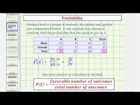
The following video shows and example of finding the probability of an event from a table.
Example 1
Suppose a study of speeding violations and drivers who use cell phones produced the following fictional data:
| Speeding violation in the last year | No speeding violation in the last year | Total | |
|---|---|---|---|
| Cell phone user | 25 | 280 | 305 |
| Not a cell phone user | 45 | 405 | 450 |
| Total | 70 | 685 | 755 |
The total number of people in the sample is 755. The row totals are 305 and 450. The column totals are 70 and 685. Notice that 305 + 450 = 755 and 70 + 685 = 755.
Calculate the following probabilities using the table.
- Find P(Person is a car phone user).
[reveal-answer q=”339376″]Show Answer[/reveal-answer]
[hidden-answer a=”339376″][/hidden-answer]
- Find P(person had no violation in the last year).
[reveal-answer q=”754811″]Show Answer[/reveal-answer]
[hidden-answer a=”754811″][/hidden-answer]
- Find P(Person had no violation in the last year AND was a car phone user).
[reveal-answer q=”490731″]Show Answer[/reveal-answer]
[hidden-answer a=”490731″][/hidden-answer]
- Find P(Person is a car phone user OR person had no violation in the last year).
[reveal-answer q=”896088″]Show Answer[/reveal-answer]
[hidden-answer a=”896088″][/hidden-answer]
- Find P(Person is a car phone user GIVEN person had a violation in the last year).
[reveal-answer q=”56218″]Show Answer[/reveal-answer]
[hidden-answer a=”56218″](The sample space is reduced to the number of persons who had a violation.)[/hidden-answer]
- Find P(Person had no violation last year GIVEN person was not a car phone user)
[reveal-answer q=”478035″]Show Answer[/reveal-answer]
[hidden-answer a=”478035″](The sample space is reduced to the number of persons who were not car phone users.)[/hidden-answer]
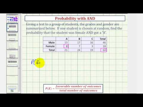
This video shows an example of how to determine the probability of an AND event using a contingency table.
Try It
This table shows the number of athletes who stretch before exercising and how many had injuries within the past year.
| Injury in last year | No injury in last year | Total | |
|---|---|---|---|
| Stretches | 55 | 295 | 350 |
| Does not stretch | 231 | 219 | 450 |
| Total | 286 | 514 | 800 |
- What is P(athlete stretches before exercising)?
[reveal-answer q=”215573″]Show Answer[/reveal-answer]
[hidden-answer a=”215573″]P(athlete stretches before exercising) == 0.4375[/hidden-answer]
- What is P(athlete stretches before exercising|no injury in the last year)?
[reveal-answer q=”399010″]Show Answer[/reveal-answer]
[hidden-answer a=”399010″]P(athlete stretches before exercising|no injury in the last year) == 0.5739[/hidden-answer]
Example 2
This table shows a random sample of 100 hikers and the areas of hiking they prefer.
Hiking Area Preference
| Sex | The Coastline | Near Lakes and Streams | On Mountain Peaks | Total |
|---|---|---|---|---|
| Female | 18 | 16 | ___ | 45 |
| Male | ___ | ___ | 14 | 55 |
| Total | ___ | 41 | ___ | ___ |
- Complete the table.
[reveal-answer q=”251999″]Show Answer[/reveal-answer]
[hidden-answer a=”251999″]Hiking Area PreferenceSex The Coastline Near Lakes and Streams On Mountain Peaks Total Female 18 16 11 45 Male 16 25 14 55 Total 34 41 25 100 [/hidden-answer]
- Are the events “being female” and “preferring the coastline” independent events?
Hint:
Let F = being female and let C = preferring the coastline.
Check if P(F AND C) = P(F) * P(C).
If P(F AND C) = P(F) * P(C), then F and C are independent.
If P(F AND C)P(F) * P(C), then F and C are not independent.
[reveal-answer q=”154586″]Show Answer[/reveal-answer]
[hidden-answer a=”154586″]
P(F AND C) == 0.18
P(F) * P(C) == (0.45)(0.34) = 0.153
P(F AND C) ≠ P(F) * P(C), so the events F and C are not independent.[/hidden-answer] - Find the probability that a person is male given that the person prefers hiking near lakes and streams.
Hint:
Let M = being male, and let L = prefers hiking near lakes and streams.
- What word tells you this is a conditional?
- Fill in the blanks and calculate the probability: P(___|___) = ___.
- Is the sample space for this problem all 100 hikers? If not, what is it?
[reveal-answer q=”146428″]Show Answer[/reveal-answer]
[hidden-answer a=”146428″]
The word given tells you that this is a conditional.
No, the sample space for this problem is the 41 hikers who prefer lakes and streams.[/hidden-answer] - Find the probability that a person is female or prefers hiking on mountain peaks.
Hint:
Let F = being female, and let P = prefers mountain peaks.
- Find P(F).
- Find P(P).
- Find P(F AND P).
- Find P(F OR P).
[reveal-answer q=”135608″]Show Answer[/reveal-answer]
[hidden-answer a=”135608″]The probability that a person is female or prefers hiking on mountain peaks =- P(F) =
- P(P) =
- P(F AND P) =
- P(F OR P) =
[/hidden-answer]
Try It
This table shows a random sample of 200 cyclists and the routes they prefer. Let M = males and H = hilly path.
| Gender | Lake Path | Hilly Path | Wooded Path | Total |
|---|---|---|---|---|
| Female | 45 | 38 | 27 | 110 |
| Male | 26 | 52 | 12 | 90 |
| Total | 71 | 90 | 39 | 200 |
- Out of the males, what is the probability that the cyclist prefers a hilly path?
[reveal-answer q=”243642″]Show Answer[/reveal-answer]
[hidden-answer a=”243642″]P(H|M) == 0.5778[/hidden-answer]
- Are the events “being male” and “preferring the hilly path” independent events?
[reveal-answer q=”945795″]Show Answer[/reveal-answer]
[hidden-answer a=”945795″]
For M and H to be independent, show P(H|M) = P(H)
P(H|M) = 0.5778, P(H) == 0.45
P(H|M)P(H), so M and H are not independent.[/hidden-answer]
Example 3
Muddy Mouse lives in a cage with three doors.
If Muddy goes out the first door, the probability that he gets caught by Alissa the cat is and the probability he is not caught is
.
If he goes out the second door, the probability he gets caught by Alissa is and the probability he is not caught is
.
The probability that Alissa catches Muddy coming out of the third door is and the probability she does not catch Muddy is
.
It is equally likely that Muddy will choose any of the three doors so the probability of choosing each door is .
Door Choice
| Caught or Not | Door One | Door Two | Door Three | Total |
|---|---|---|---|---|
| Caught | ____ | |||
| Not Caught | ____ | |||
| Total | ____ | ____ | ____ | 1 |
- The first entry
is P(Door One AND Caught)
- The entry
is P(Door One AND Not Caught)
Verify the remaining entries.
- Complete the probability contingency table. Calculate the entries for the totals. Verify that the lower-right corner entry is 1.
[reveal-answer q=”135107″]Show Answer[/reveal-answer]
[hidden-answer a=”135107″]
Door ChoiceCaught or Not Door One Door Two Door Three Total Caught Not Caught Total 1 [/hidden-answer]
- What is the probability that Alissa does not catch Muddy?
[reveal-answer q=”565264″]Show Answer[/reveal-answer]
[hidden-answer a=”565264″][/hidden-answer]
- What is the probability that Muddy chooses Door One OR Door Two given that Muddy is caught by Alissa?
[reveal-answer q=”404174″]Show Answer[/reveal-answer]
[hidden-answer a=”404174″][/hidden-answer]
Example 4
This table contains the number of crimes per 100,000 inhabitants from 2008 to 2011 in the U.S.
United States Crime Index Rates Per 100,000 Inhabitants 2008–2011
| Year | Robbery | Burglary | Rape | Vehicle | Total |
|---|---|---|---|---|---|
| 2008 | 145.7 | 732.1 | 29.7 | 314.7 | |
| 2009 | 133.1 | 717.7 | 29.1 | 259.2 | |
| 2010 | 119.3 | 701 | 27.7 | 239.1 | |
| 2011 | 113.7 | 702.2 | 26.8 | 229.6 | |
| Total |
TOTAL each column and each row. Total data = 4,520.7
- Find P(2009 AND Robbery).
[reveal-answer q=”19793″]Show Answer[/reveal-answer]
[hidden-answer a=”19793″]0.0294[/hidden-answer] - Find P(2010 AND Burglary).
[reveal-answer q=”842217″]Show Answer[/reveal-answer]
[hidden-answer a=”842217″]0.1551[/hidden-answer] - Find P(2010 OR Burglary).
[reveal-answer q=”757233″]Show Answer[/reveal-answer]
[hidden-answer a=”757233″]0.7165[/hidden-answer] - Find P(2011|Rape).
[reveal-answer q=”21461″]Show Answer[/reveal-answer]
[hidden-answer a=”21461″]0.2365[/hidden-answer] - Find P(Vehicle|2008).
[reveal-answer q=”109508″]Show Answer[/reveal-answer]
[hidden-answer a=”109508″]0.2575[/hidden-answer]
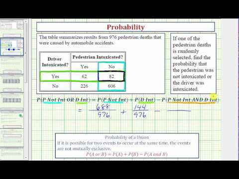
This video gives and example of determining an “OR” probability given a table.
Try It
This table relates the weights and heights of a group of individuals participating in an observational study.
| Weight/Height | Tall | Medium | Short | Totals |
|---|---|---|---|---|
| Obese | 18 | 28 | 14 | |
| Normal | 20 | 51 | 28 | |
| Underweight | 12 | 25 | 9 | |
| Totals |
- Find the total for each row and column.
[reveal-answer q=”507433″]Show Answer[/reveal-answer]
[hidden-answer a=”507433″]Weight/Height Tall Medium Short Totals Obese 18 28 14 60 Normal 20 51 28 99 Underweight 12 25 9 46 Totals 50 104 51 205 [/hidden-answer]
- Find the probability that a randomly chosen individual from this group is Tall.
[reveal-answer q=”370094″]Show Answer[/reveal-answer]
[hidden-answer a=”370094″]P(Tall) == 0.244[/hidden-answer]
- Find the probability that a randomly chosen individual from this group is Obese and Tall.
[reveal-answer q=”850929″]Show Answer[/reveal-answer]
[hidden-answer a=”850929″]P(Obese AND Tall) == 0.088[/hidden-answer]
- Find the probability that a randomly chosen individual from this group is Tall given that the idividual is Obese.
[reveal-answer q=”94869″]Show Answer[/reveal-answer]
[hidden-answer a=”94869″]P(Tall|Obese) == 0.3[/hidden-answer]
- Find the probability that a randomly chosen individual from this group is Obese given that the individual is Tall.
[reveal-answer q=”829472″]Show Answer[/reveal-answer]
[hidden-answer a=”829472″]P(Obese|Tall) == 0.36[/hidden-answer]
- Find the probability a randomly chosen individual from this group is Tall and Underweight.
[reveal-answer q=”76983″]Show Answer[/reveal-answer]
[hidden-answer a=”76983″]P(Tall AND Underweight == 0.0585[/hidden-answer]
- Are the events Obese and Tall independent?
[reveal-answer q=”765225″]Show Answer[/reveal-answer]
[hidden-answer a=”765225″]No. P(Tall)(Tall|Obese).[/hidden-answer]
References
“Blood Types.” American Red Cross, 2013. Available online at http://www.redcrossblood.org/learn-a...od/blood-types (accessed May 3, 2013).
Data from the National Center for Health Statistics, part of the United States Department of Health and Human Services.
Data from United States Senate. Available online at www.senate.gov (accessed May 2, 2013).
Haiman, Christopher A., Daniel O. Stram, Lynn R. Wilkens, Malcom C. Pike, Laurence N. Kolonel, Brien E. Henderson, and Loīc Le Marchand. “Ethnic and Racial Differences in the Smoking-Related Risk of Lung Cancer.” The New England Journal of Medicine, 2013. Available online at http://www.nejm.org/doi/full/10.1056/NEJMoa033250 (accessed May 2, 2013).
“Human Blood Types.” Unite Blood Services, 2011. Available online at http://www.unitedbloodservices.org/learnMore.aspx (accessed May 2, 2013).
Samuel, T. M. “Strange Facts about RH Negative Blood.” eHow Health, 2013. Available online at http://www.ehow.com/facts_5552003_st...ive-blood.html (accessed May 2, 2013).
“United States: Uniform Crime Report – State Statistics from 1960–2011.” The Disaster Center. Available online at http://www.disastercenter.com/crime/ (accessed May 2, 2013).
Concept Review
There are several tools you can use to help organize and sort data when calculating probabilities. Contingency tables help display data and are particularly useful when calculating probabilites that have multiple dependent variables.
- OpenStax, Statistics, Contingency Tables. Provided by: OpenStax. Located at: http://cnx.org/contents/30189442-6998-4686-ac05-ed152b91b9de@17.34:22/Introductory_Statistics. License: CC BY: Attribution
- Introductory Statistics . Authored by: Barbara Illowski, Susan Dean. Provided by: Open Stax. Located at: http://cnx.org/contents/30189442-6998-4686-ac05-ed152b91b9de@17.44. License: CC BY: Attribution. License Terms: Download for free at http://cnx.org/contents/30189442-699...2b91b9de@17.44
- Ex: Determine a Probability with AND using a Table . Authored by: Mathispower4u. Located at: https://youtu.be/Xp-Hm2ufaYE. License: All Rights Reserved. License Terms: Standard YouTube License
- Ex: Basic Example of Finding Probability From a Table. Authored by: Mathispower4u. Located at: https://youtu.be/O6obluO7FTQ. License: All Rights Reserved. License Terms: Standard YouTube LIcense
- Ex: Determine the Probability of a Union Using a Table - Not Mutually Exclusive. Authored by: Mathispower4u. Located at: https://youtu.be/sbJXS9etEKw. License: All Rights Reserved. License Terms: Standard YouTube License


