7.9: Introduction to Inequalities and Interval Notation

Learning Objectives

• Understand interval notation.
• Determine when intervals are open or closed.
• Graph the solutions of an inequality on a number line and express the solutions using interval notation.

Unbounded Intervals

An algebraic inequality, such as \(x≥2\), is read “\(x\) is greater than or equal to \(2\).” This inequality has infinitely many solutions for \(x\). Some of the solutions are \(2, 3, 3.5, 5, 20,\) and \(20.001\). Since it is impossible to list all of the solutions, a system is needed that allows a clear communication of this infinite set. Two common ways of expressing solutions to an inequality are by graphing them on a number line and using interval notation.

To express the solution graphically, draw a number line and shade in all the values that are solutions to the inequality. Interval notation is textual and uses specific notation as follows:

Figure \(\PageIndex{1}\)

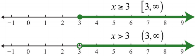
Determine the interval notation after graphing the solution set on a number line. The numbers in interval notation should be written in the same order as they appear on the number line, with smaller numbers in the set appearing first. In this example, there is an inclusive inequality, which means that the lower-bound 2 is included in the solution. Denote this with a closed dot on the number line and a square bracket in interval notation. The symbol (∞) is read as infinity and indicates that the set is unbounded to the right on a number line. Interval notation requires a parenthesis to enclose infinity. The square bracket indicates the boundary is included in the solution. The parentheses indicate the boundary is not included. Infinity is an upper bound to the real numbers, but is not itself a real number: it cannot be included in the solution set.

Now compare the interval notation in the previous example to that of the strict, or noninclusive, inequality that follows:

Figure \(\PageIndex{2}\)

Strict inequalities imply that solutions may get very close to the boundary point, in this case 2, but not actually include it. Denote this idea with an open dot on the number line and a round parenthesis in interval notation.

Example \(\PageIndex{1}\)

Graph and give the interval notation equivalent:

\(x<3\).

Solution:

Use an open dot at \(3\) and shade all real numbers strictly less than \(3\). Use negative infinity \((−∞)\) to indicate that the solution set is unbounded to the left on a number line.

Figure \(\PageIndex{3}\)

Answer:

Interval notation: \((-∞, 3)\)

Example \(\PageIndex{2}\)

Graph and give the interval notation equivalent:

\(x≤5\).

Solution:

Use a closed dot and shade all numbers less than and including 5.

Figure \(\PageIndex{4}\)

Answer:

Interval notation: \((−∞, 5]\)

It is important to see that \(5≥x\) is the same as \(x≤5\). Both require values of \(x\) to be smaller than or equal to \(5\). To avoid confusion, it is good practice to rewrite all inequalities with the variable on the left.

 

In summary,

Figure \(\PageIndex{5}\)

Figure \(\PageIndex{6}\)

Bounded Intervals

An inequality such as

\(-1\leq x<3\)

reads “negative one is less than or equal to \(x\) and \(x\) is less than three.” This is a compound inequality because it can be decomposed as follows:

\(-1\leq x\) and \(x<3\)

The logical “and” requires that both conditions must be true. Both inequalities are satisfied by all the elements in the intersection, denoted \(∩\), of the solution sets of each.

Alternatively, we may interpret \(−1≤x<3\) as all possible values for \(x\) between or bounded by \(−1\) and \(3\) on a number line. For example, one such solution is \(x=1\). Notice that \(1\) is between \(−1\) and \(3\) on a number line, or that \(−1 < 1 < 3\). Similarly, we can see that other possible solutions are \(−1, −0.99, 0, 0.0056, 1.8\), and \(2.99\). Since there are infinitely many real numbers between \(−1\) and \(3\), we must express the solution graphically and/or with interval notation, in this case \([−1, 3)\).

Example \(\PageIndex{3}\)

Graph and give the interval notation equivalent:

\(−\frac{3}{2}<x<2\).

Solution:

Shade all real numbers bounded by, or strictly between, \(−\frac{3}{2}=−1\frac{1}{2}\) and \(2\).

Figure \(\PageIndex{7}\)

Answer:

Interval notation: \((−\frac{3}{2}, 2)\)

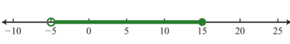
Example \(\PageIndex{7}\)

Graph and give the interval notation equivalent:

\(−5<x\leq 15\)

Solution:

Shade all real numbers between \(−5\) and \(15\), and indicate that the upper bound, \(15\), is included in the solution set by using a closed dot.

Figure \(\PageIndex{8}\)

Answer:

Interval notation: \((−5, 15]\)

In the previous two examples, we did not decompose the inequalities; instead we chose to think of all real numbers between the two given bounds.

In summary,

Figure \(\PageIndex{9}\)

Key Takeaways

• Inequalities usually have infinitely many solutions, so rather than presenting an impossibly large list, we present such solutions sets either graphically on a number line or textually using interval notation.
• Inclusive inequalities with the “or equal to” component are indicated with a closed dot on the number line and with a square bracket using interval notation.
• Strict inequalities without the “or equal to” component are indicated with an open dot on the number line and a parenthesis using interval notation.
• Compound inequalities of the form \(m<x<n\) can be decomposed into two inequalities using the logical “and.” However, it is just as valid to consider the argument \(x\) to be bounded between the values \(m\) and \(n\).