9.4: Applications of Normal Distributions

Learning Objectives

• Apply the characteristics of a normal distribution to solve application problems

Introduction

This section will cover some of the types of questions that can be answered using the properties of a normal distribution. The first examples deal with more theoretical questions that will help you master basic understandings and computational skills, while the later problems will provide examples with real data, or at least a real context.

Normal Distributions with Real Data

The foundation of performing experiments by collecting surveys and samples is most often based on the normal distribution. Here are two examples to get you started.

Example \(\PageIndex{1}\)

The Information Centre of the National Health Service in Britain collects and publishes a great deal of information and statistics on health issues affecting the population. One such comprehensive data set tracks information about the health of children [1]. According to its statistics, in 2006, the mean height of 12-year-old boys was 152.9 cm, with a standard deviation of 8.5 cm. If 12-year-old Cecil is 158 cm, approximately what percentage of all 12-year-old boys in Britain is he taller than?

Solution

We first must assume that the height of 12-year-old boys in Britain is normally distributed, and this seems like a reasonable assumption to make. We need to find the percentage, or probability, of a 12-year-old boy being shorter than 158 cm, i.e., \(P(X < 158)\). We let \(x = 158\) and calculate the z-score:

\(z = \dfrac{x-\mu}{\sigma}\)

\(z = \dfrac{158-152.9}{8.5}\)

\(z = 0.6\)

As always, draw a sketch and estimate a reasonable answer prior to calculating the percentage.

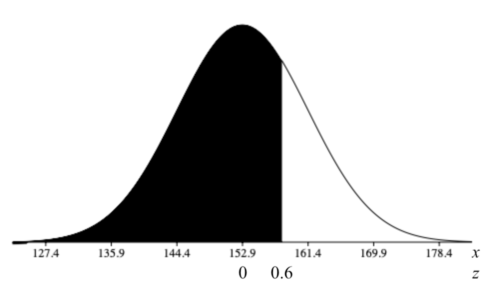
From the table, the probability is \(P(Z < 0.6) = 0.7257\). We would estimate that Cecil is taller than about 73% of 12-year-old boys. We could also phrase our assumption this way: the probability of a randomly selected British 12- year-old boy being shorter than Cecil is about 0.73. Often with data like this, we use percentiles. We would say that Cecil is in the 73^rd percentile for height among 12-year-old boys in Britain.

Example \(\PageIndex{2}\)

Suppose that the distribution of the mass of female marine iguanas in Puerto Villamil in the Galapagos Islands is approximately normal, with a mean mass of 950 g and a standard deviation of 325 g. There are very few young marine iguanas in the populated areas of the islands because feral cats tend to kill them. How rare is it that we would find a female marine iguana with a mass less than 400 g in this area?

Solution

We need to find the probability of a female marine iguana being less than 400 grams, i.e., \(P(X < 400)\). We let \(x = 400\) and calculate the z-score:

\(z = \dfrac{x-\mu}{\sigma}\)

\(z = \dfrac{400-950}{325}\)

\(z \approx -1.69\)

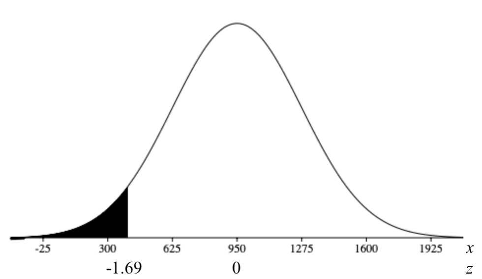
We need to find \(P(Z < -1.69)\). Using the table, we obtain a probability of \(0.0455\). With a probability of approximately 0.0455, or only about 5%, we could say it is rather unlikely that we would find an iguana this small.

Try It \(\PageIndex{1}\)

A candy company sells small bags of candy and attempts to keep the number of pieces in each bag the same, though small differences due to random variation in the packaging process lead to different amounts in individual packages. A quality control expert from the company has determined that the mean number of pieces in each bag is normally distributed, with a mean of 57.3 and a standard deviation of 1.2. Endy opened a bag of candy and felt he was cheated. His bag contained only 55 candies. Does Endy have reason to complain?

Answer

To determine if Endy was cheated, we need to find the probability of selecting a bag of candy with 55 or fewer candies, i.e., \(P(X \leq 55)\

). We let \(x = 55\) and calculate the z-score:

\(z = \dfrac{x-\mu}{\sigma}\)

\(z = \dfrac{55-57.3}{1.2}\)

\(z \approx -1.92\)

Next, we can draw a figure to see the shaded region:

We need to find \(P(Z < -1.92)\). Using the table, we obtain a probability of \(0.0274\). Hence, there is about a 3% chance that he would get a bag of candy with 55 or fewer pieces, so Endy should feel cheated because the chances of getting a bag with 55 or fewer candies is so low.

Example \(\PageIndex{3}\)

The physical plant at the main campus of a large state university receives daily requests to replace florescent light bulbs. The distribution of the number of daily requests is bell-shaped and has a mean of 59 and a standard deviation of 9. What is the percentage of light bulb replacement requests numbering between 59 and 77?

Solution

We need to calculate \(P(59 < X < 77)\) given \(\mu = 59\) and \(\sigma = 9\). Re-writing the probability with z-scores:

\[P(59 < X < 77) = P\left( \dfrac{59 - 59}{9} < Z < \dfrac{77 - 59}{9} \right) = P(0 < Z < 2) \nonumber\]

Using the table, the probability is \(0.9772 - 0.5000 = 0.4772\). Thus, \(47.72\%\) of daily light bulb replacement requests number between 59 and 77.

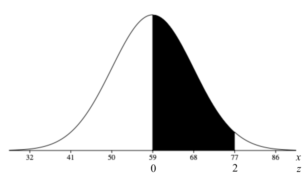
Note: this problem could have been approximated using the Empirical Rule.

Try It \(\PageIndex{2}\)

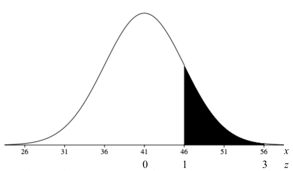
A company has a policy of retiring company cars; this policy looks at number of miles driven, purpose of trips, style of car and other features. The distribution of the number of months in service for the fleet of cars is bell-shaped and has a mean of 41 months and a standard deviation of 5 months. What is the percentage of cars that remain in service between 46 and 56 months?

Answer

We need to calculate \(P(46 < X < 56)\) given \(\mu = 41\) and \(\sigma = 5\). Re-writing the probability with z-scores:

\[P(46 < X < 56) = P\left( \dfrac{46 - 41}{5} < Z < \dfrac{56 - 41}{5} \right) = P(1 < Z < 3) \nonumber\]

Using the table, the probability is \(0.9987 - 0.8413 = 0.1574\). Thus, \(15.74\%\) of cars remain in service between 46 and 56 months.

Note: this problem could also have been approximated using the Empirical Rule.