
9.3: Probability Computations for General Normal Distributions
- Page ID
- 30311
\( \newcommand{\vecs}[1]{\overset { \scriptstyle \rightharpoonup} {\mathbf{#1}} } \)
\( \newcommand{\vecd}[1]{\overset{-\!-\!\rightharpoonup}{\vphantom{a}\smash {#1}}} \)
\( \newcommand{\id}{\mathrm{id}}\) \( \newcommand{\Span}{\mathrm{span}}\)
( \newcommand{\kernel}{\mathrm{null}\,}\) \( \newcommand{\range}{\mathrm{range}\,}\)
\( \newcommand{\RealPart}{\mathrm{Re}}\) \( \newcommand{\ImaginaryPart}{\mathrm{Im}}\)
\( \newcommand{\Argument}{\mathrm{Arg}}\) \( \newcommand{\norm}[1]{\| #1 \|}\)
\( \newcommand{\inner}[2]{\langle #1, #2 \rangle}\)
\( \newcommand{\Span}{\mathrm{span}}\)
\( \newcommand{\id}{\mathrm{id}}\)
\( \newcommand{\Span}{\mathrm{span}}\)
\( \newcommand{\kernel}{\mathrm{null}\,}\)
\( \newcommand{\range}{\mathrm{range}\,}\)
\( \newcommand{\RealPart}{\mathrm{Re}}\)
\( \newcommand{\ImaginaryPart}{\mathrm{Im}}\)
\( \newcommand{\Argument}{\mathrm{Arg}}\)
\( \newcommand{\norm}[1]{\| #1 \|}\)
\( \newcommand{\inner}[2]{\langle #1, #2 \rangle}\)
\( \newcommand{\Span}{\mathrm{span}}\) \( \newcommand{\AA}{\unicode[.8,0]{x212B}}\)
\( \newcommand{\vectorA}[1]{\vec{#1}} % arrow\)
\( \newcommand{\vectorAt}[1]{\vec{\text{#1}}} % arrow\)
\( \newcommand{\vectorB}[1]{\overset { \scriptstyle \rightharpoonup} {\mathbf{#1}} } \)
\( \newcommand{\vectorC}[1]{\textbf{#1}} \)
\( \newcommand{\vectorD}[1]{\overrightarrow{#1}} \)
\( \newcommand{\vectorDt}[1]{\overrightarrow{\text{#1}}} \)
\( \newcommand{\vectE}[1]{\overset{-\!-\!\rightharpoonup}{\vphantom{a}\smash{\mathbf {#1}}}} \)
\( \newcommand{\vecs}[1]{\overset { \scriptstyle \rightharpoonup} {\mathbf{#1}} } \)
\( \newcommand{\vecd}[1]{\overset{-\!-\!\rightharpoonup}{\vphantom{a}\smash {#1}}} \)
- Compute probabilities for any normal distribution using the Z table
In most practical problems involving normal distributions, the curve will not be as we have seen so far, with \(\mu=0\) and \(\sigma =1\). When using a Z table, you will first have to standardize the distribution by calculating the z-score(s).
Standardizing a data value, \(x\), is the process of converting it to a z-score using the formula \(z = \dfrac{x - \mu}{\sigma}\).
To compute a probability of the form \(P(a<X<b)\) we use the following process.
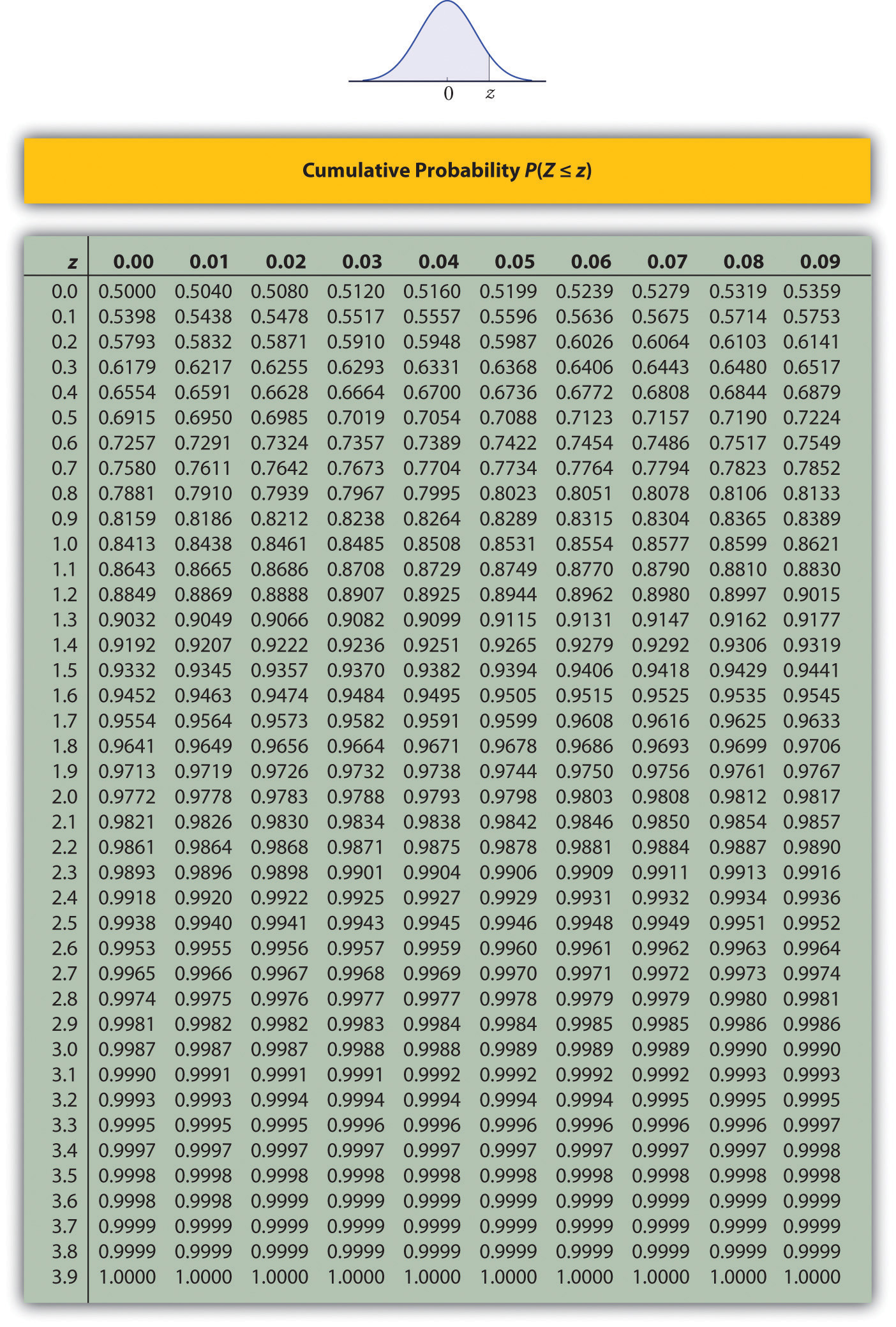
If \(X\) is normally distributed with mean \(\mu\) and standard deviation \(\sigma\), then \[P(a<X<b)=P\left ( \dfrac{a-\mu }{\sigma }<Z<\dfrac{b-\mu }{\sigma } \right ) \nonumber\] where \(Z\) denotes a standard normal distribution. \(a\) can be any decimal number or \(-\infty\); \(b\) can be any decimal number or \(\infty\).
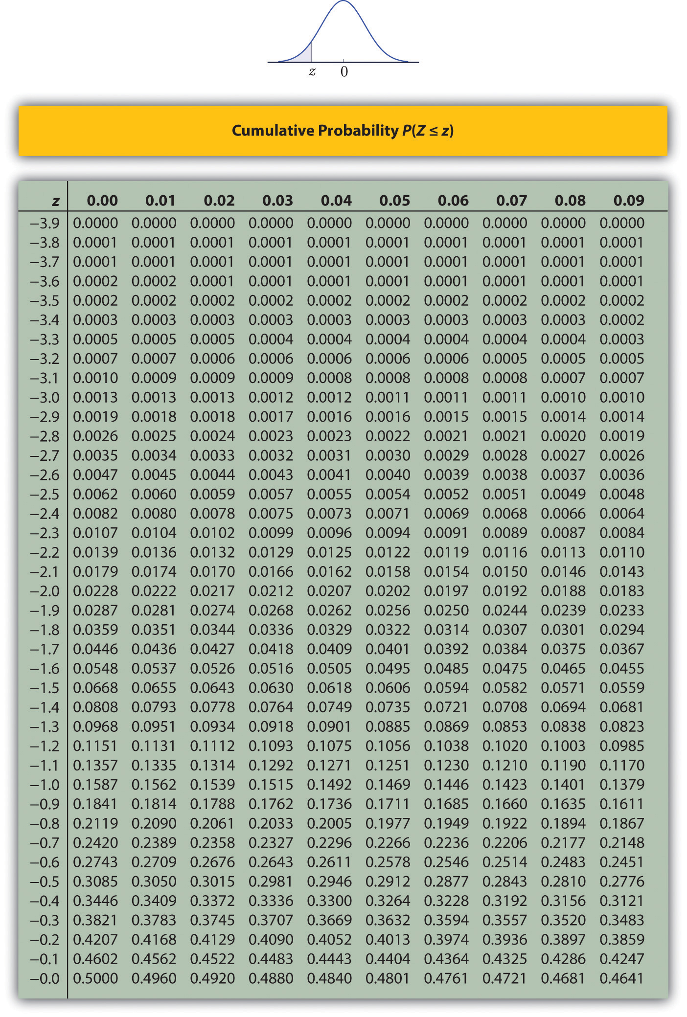
The table can also be found online here in section 6.
The new endpoints \(\dfrac{(a-\mu )}{\sigma }\) and \(\dfrac{(b-\mu )}{\sigma }\) are the \(z\)-scores of \(a\) and \(b\).
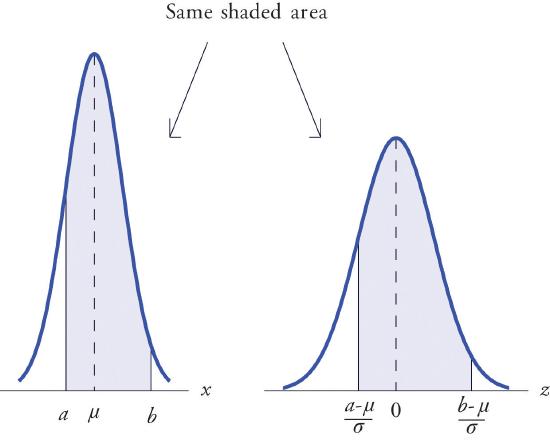
The figure below illustrates the meaning of the process geometrically: the two shaded regions, one under the curve for \(X\) and the other under the curve for \(Z\), have the same area. Instead of drawing both bell curves, though, we will draw a single generic bell-shaped curve with both an \(x\)-axis and a \(z\)-axis below it.
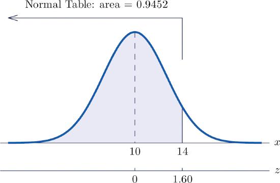
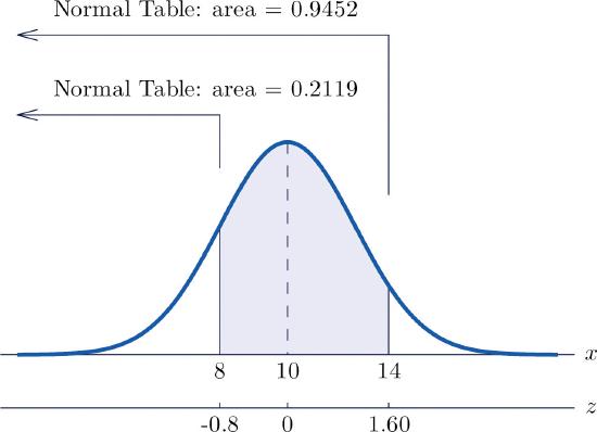
Let \(X\) be normally distributed with mean \(\mu =10\) and standard deviation \(\sigma =2.5\). Compute the following probabilities.
- \(P(X<14)\).
- \(P(8<X<14)\).
Solution:
- See the figure below. \[\begin{align*} P(X<14) &= P\left ( Z<\dfrac{14-\mu }{\sigma } \right )\\ &= P\left ( Z<\dfrac{14-10}{2.5} \right )\\ &= P(Z<1.60)\\ &= 0.9452 \end{align*}\]
- See the figure below. \[\begin{align*} P(8<X<14) &= P\left ( \dfrac{8-10}{2.5}<Z<\dfrac{14-10}{2.5} \right )\\ &= P\left ( -0.80<Z<1.60 \right )\\ &= 0.9452-0.2119\\ &= 0.7333 \end{align*}\]
Let \(X\) be normally distributed with mean \(37.5\) and standard deviation \(4.5\). Find the probability that \(X\) will be between \(30\) and \(40\).
- Answer
-
For \(X\), \(\mu =37.5\) and \(\sigma =4.5\). The problem is to compute \(P(30<X<40)\). The figure below illustrates the following computation:
\[\begin{align*} P(30<X<40) &= P\left ( \dfrac{30-\mu }{\sigma }<Z<\dfrac{40-\mu }{\sigma } \right )\\ &= P\left ( \dfrac{30-37.5}{4.5}<Z<\dfrac{40-37.5}{4.5} \right )\\ &= P\left ( -1.67<Z<0.56\right )\\ &= 0.7123-0.0475\\ &= 0.6648 \end{align*}\]
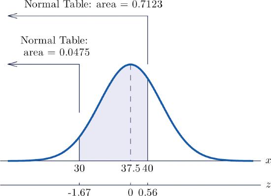
Note that the two \(z\)-scores were rounded to two decimal places in order to use the table.
Let \(X\) be normally distributed with mean \(510\) and standard deviation \(60\). Find the percentage of data values that exceed 650.
Solution:
\(X\) is normally distributed with mean \(\mu = 510\) and standard deviation \(\sigma = 60\). The probability that \(X\) lies in a particular interval is the same as the proportion or percent of all data values that lie in that interval. Thus the solution to the problem is \(P(X>650)\), expressed as a percentage. The figure below illustrates the following computation:
\[\begin{align*} P(X>650) &= P\left ( Z>\dfrac{650-\mu }{\sigma } \right )\\ &= P\left ( Z>\dfrac{650-510}{60} \right )\\ &= P(Z>2.33)\\ &= 1-0.9901\\ &= 0.0099 \end{align*}\]
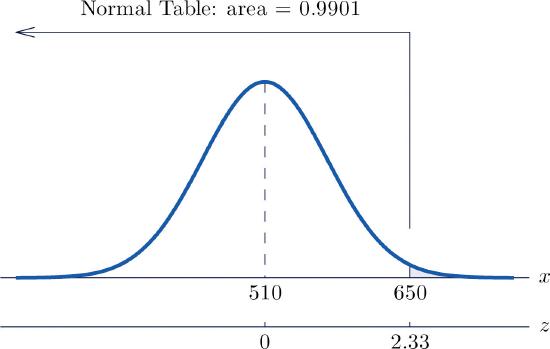
The percent of all data values that exceed \(650\) is \(0.0099\), hence \(0.99\%\) or about \(1\%\).
Contributor
Anonymous