
Ch 6.2 Application of Normal Distribution
- Page ID
- 15902
\( \newcommand{\vecs}[1]{\overset { \scriptstyle \rightharpoonup} {\mathbf{#1}} } \)
\( \newcommand{\vecd}[1]{\overset{-\!-\!\rightharpoonup}{\vphantom{a}\smash {#1}}} \)
\( \newcommand{\dsum}{\displaystyle\sum\limits} \)
\( \newcommand{\dint}{\displaystyle\int\limits} \)
\( \newcommand{\dlim}{\displaystyle\lim\limits} \)
\( \newcommand{\id}{\mathrm{id}}\) \( \newcommand{\Span}{\mathrm{span}}\)
( \newcommand{\kernel}{\mathrm{null}\,}\) \( \newcommand{\range}{\mathrm{range}\,}\)
\( \newcommand{\RealPart}{\mathrm{Re}}\) \( \newcommand{\ImaginaryPart}{\mathrm{Im}}\)
\( \newcommand{\Argument}{\mathrm{Arg}}\) \( \newcommand{\norm}[1]{\| #1 \|}\)
\( \newcommand{\inner}[2]{\langle #1, #2 \rangle}\)
\( \newcommand{\Span}{\mathrm{span}}\)
\( \newcommand{\id}{\mathrm{id}}\)
\( \newcommand{\Span}{\mathrm{span}}\)
\( \newcommand{\kernel}{\mathrm{null}\,}\)
\( \newcommand{\range}{\mathrm{range}\,}\)
\( \newcommand{\RealPart}{\mathrm{Re}}\)
\( \newcommand{\ImaginaryPart}{\mathrm{Im}}\)
\( \newcommand{\Argument}{\mathrm{Arg}}\)
\( \newcommand{\norm}[1]{\| #1 \|}\)
\( \newcommand{\inner}[2]{\langle #1, #2 \rangle}\)
\( \newcommand{\Span}{\mathrm{span}}\) \( \newcommand{\AA}{\unicode[.8,0]{x212B}}\)
\( \newcommand{\vectorA}[1]{\vec{#1}} % arrow\)
\( \newcommand{\vectorAt}[1]{\vec{\text{#1}}} % arrow\)
\( \newcommand{\vectorB}[1]{\overset { \scriptstyle \rightharpoonup} {\mathbf{#1}} } \)
\( \newcommand{\vectorC}[1]{\textbf{#1}} \)
\( \newcommand{\vectorD}[1]{\overrightarrow{#1}} \)
\( \newcommand{\vectorDt}[1]{\overrightarrow{\text{#1}}} \)
\( \newcommand{\vectE}[1]{\overset{-\!-\!\rightharpoonup}{\vphantom{a}\smash{\mathbf {#1}}}} \)
\( \newcommand{\vecs}[1]{\overset { \scriptstyle \rightharpoonup} {\mathbf{#1}} } \)
\(\newcommand{\longvect}{\overrightarrow}\)
\( \newcommand{\vecd}[1]{\overset{-\!-\!\rightharpoonup}{\vphantom{a}\smash {#1}}} \)
\(\newcommand{\avec}{\mathbf a}\) \(\newcommand{\bvec}{\mathbf b}\) \(\newcommand{\cvec}{\mathbf c}\) \(\newcommand{\dvec}{\mathbf d}\) \(\newcommand{\dtil}{\widetilde{\mathbf d}}\) \(\newcommand{\evec}{\mathbf e}\) \(\newcommand{\fvec}{\mathbf f}\) \(\newcommand{\nvec}{\mathbf n}\) \(\newcommand{\pvec}{\mathbf p}\) \(\newcommand{\qvec}{\mathbf q}\) \(\newcommand{\svec}{\mathbf s}\) \(\newcommand{\tvec}{\mathbf t}\) \(\newcommand{\uvec}{\mathbf u}\) \(\newcommand{\vvec}{\mathbf v}\) \(\newcommand{\wvec}{\mathbf w}\) \(\newcommand{\xvec}{\mathbf x}\) \(\newcommand{\yvec}{\mathbf y}\) \(\newcommand{\zvec}{\mathbf z}\) \(\newcommand{\rvec}{\mathbf r}\) \(\newcommand{\mvec}{\mathbf m}\) \(\newcommand{\zerovec}{\mathbf 0}\) \(\newcommand{\onevec}{\mathbf 1}\) \(\newcommand{\real}{\mathbb R}\) \(\newcommand{\twovec}[2]{\left[\begin{array}{r}#1 \\ #2 \end{array}\right]}\) \(\newcommand{\ctwovec}[2]{\left[\begin{array}{c}#1 \\ #2 \end{array}\right]}\) \(\newcommand{\threevec}[3]{\left[\begin{array}{r}#1 \\ #2 \\ #3 \end{array}\right]}\) \(\newcommand{\cthreevec}[3]{\left[\begin{array}{c}#1 \\ #2 \\ #3 \end{array}\right]}\) \(\newcommand{\fourvec}[4]{\left[\begin{array}{r}#1 \\ #2 \\ #3 \\ #4 \end{array}\right]}\) \(\newcommand{\cfourvec}[4]{\left[\begin{array}{c}#1 \\ #2 \\ #3 \\ #4 \end{array}\right]}\) \(\newcommand{\fivevec}[5]{\left[\begin{array}{r}#1 \\ #2 \\ #3 \\ #4 \\ #5 \\ \end{array}\right]}\) \(\newcommand{\cfivevec}[5]{\left[\begin{array}{c}#1 \\ #2 \\ #3 \\ #4 \\ #5 \\ \end{array}\right]}\) \(\newcommand{\mattwo}[4]{\left[\begin{array}{rr}#1 \amp #2 \\ #3 \amp #4 \\ \end{array}\right]}\) \(\newcommand{\laspan}[1]{\text{Span}\{#1\}}\) \(\newcommand{\bcal}{\cal B}\) \(\newcommand{\ccal}{\cal C}\) \(\newcommand{\scal}{\cal S}\) \(\newcommand{\wcal}{\cal W}\) \(\newcommand{\ecal}{\cal E}\) \(\newcommand{\coords}[2]{\left\{#1\right\}_{#2}}\) \(\newcommand{\gray}[1]{\color{gray}{#1}}\) \(\newcommand{\lgray}[1]{\color{lightgray}{#1}}\) \(\newcommand{\rank}{\operatorname{rank}}\) \(\newcommand{\row}{\text{Row}}\) \(\newcommand{\col}{\text{Col}}\) \(\renewcommand{\row}{\text{Row}}\) \(\newcommand{\nul}{\text{Nul}}\) \(\newcommand{\var}{\text{Var}}\) \(\newcommand{\corr}{\text{corr}}\) \(\newcommand{\len}[1]{\left|#1\right|}\) \(\newcommand{\bbar}{\overline{\bvec}}\) \(\newcommand{\bhat}{\widehat{\bvec}}\) \(\newcommand{\bperp}{\bvec^\perp}\) \(\newcommand{\xhat}{\widehat{\xvec}}\) \(\newcommand{\vhat}{\widehat{\vvec}}\) \(\newcommand{\uhat}{\widehat{\uvec}}\) \(\newcommand{\what}{\widehat{\wvec}}\) \(\newcommand{\Sighat}{\widehat{\Sigma}}\) \(\newcommand{\lt}{<}\) \(\newcommand{\gt}{>}\) \(\newcommand{\amp}{&}\) \(\definecolor{fillinmathshade}{gray}{0.9}\)Ch 6.2 Using the Normal distribution
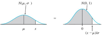
When X is normally distributed with mean μ and standard deviation σ, N( μ,σ) probability of range of X can be represented by the area under normal density curve \( y = \frac{e^{\frac{-1}{2}\cdot {(\frac{x-\mu}{\sigma})}^2}}{\sigma \sqrt{2 \pi}} \) (no need to memorize.)
The same properties of bell shape density curve apply:
Probability = area = relative frequency (percentage)
a) P( X > μ ) = 0.5, P(X < μ) = 0.5
b) P( a < X < b) = area between a and b under the density bell curve.
A) Find Probability of X in Normal distribution
Use online Normal distribution calculator to find prob.
http://onlinestatbook.com/2/calculators/normal_dist.html
Specify mean = μ, SD= σ
-For left area or P(x < a) click below
-For right area or P(x > a) click above
-For area between two values a and b P( a < x < b), click between
-For area outside of a and b, P(x <a or x > b), click outside
-Click “Recalculate”
B) Find X given probability in Normal Distribution
Use Inverse Normal Calculator to find the cut-off given a left area, right area, between area or outside area of two tails.
http://onlinestatbook.com/2/calculators/inverse_normal_dist.html
Specify area, mean= μ, SD= σ
select if area is below, above, between or outside.
Click “Recalculate”
Note: left area = bottom percentage = percentile. Right area = top percent
a) Find cutoff X for Top k percentage:
Use Inverse online calculator, above
b) Find cutoff X for Bottom k percentage or k percentile: Use Inverse online calculator, below
Ex1. Final exam of a standardized test is normally distributed with mean 63 and standard deviation 5.
a) Find the probability that a randomly selected student scored more than 65 on the exam.
Use Online Normal calculator.
Mean = 63, SD =5,
Click above, enter 65.
Recalculate
P( X > 65 ) = 0.3446.
b) Find the probability that a score less than 85
Use Online Normal calculator. Mean = 63, SD =5,
Click below, enter 85.
Recalculate
P( X < 85 ) = 1
c) Find the 90th percentile score. ( top 10%)
Use Inverse Normal Calculator, mean = 63, SD = 5
Enter Area = 0.9, Click below
The cut-off X is at the below box.
P(X < __69.4___) = 0.9. The 90th percentile is 69.4.
Ex2: Heights of men are normally distributed with mean of 68.6 in. and a standard deviation of 2.8 in.
Find the probability that a randomly selected man has a height greater than 72 in.
Use Online Normal calculator.
Mean = 68.6, sd =2.8, Click above, enter 72.
Recalculate
P(X > 72) = 0.1123
Ex3. Given pulse rate of women is normally distributed with a mean of 74 bpm and a standard deviation of 12.5 bpm. Find the pulse rates of lowest 5% and highest 5% of women.
Total area = 5% + 5% =0.1
Find cutoff pulse rate for lowest 5% and highest 5%. Use Inverse Normal calculator.
Area = 0.10, Mean = 74, SD=12.5. Click Outside.
Recalculate.
lowest 5% cutoff = 53.4 bpm highest 5%=94.6 bpm
Ex4. A circus farmer grows mandarin oranges finds that the diameters of mandarin oranges harvested on his farm follow a normal distribution with a mean diameter of 5.85 cm and standard deviation of 0.24cm.
a) Find the probability that a normally selected mandarin orange from his farm has a diameter larger than 6 cm.
Use Online Normal calculator.
Mean = 5.85, sd =0.24,
Click above, enter 6.
Recalculate
P( X > 6 ) = 0.266
b) Find the middle 20% diameter of mandarin oranges from his farm.
Use Inverse Normal Calculator
Area = 0.2, Mean = 5.85, sd=0.24
Click Between.
P( _5.79____< X < __5.91____) = 0.2
Ex5. A TV has a life that is normally distributed with a mean of 6.5 years and a standard deviation of 2.3 years. If the company offers a warranty to replace any TV within 3 years. What percent of TV will need to be replaced?
To find percent, use Normal online calculator.
Mean = 6.5 , sd =2.3,
Click below, enter 3.
Recalculate
P (X < 3) = 0.064 = 6.4%