
Ch 2.7 Measure of Spread and Variation
- Page ID
- 15885
\( \newcommand{\vecs}[1]{\overset { \scriptstyle \rightharpoonup} {\mathbf{#1}} } \)
\( \newcommand{\vecd}[1]{\overset{-\!-\!\rightharpoonup}{\vphantom{a}\smash {#1}}} \)
\( \newcommand{\id}{\mathrm{id}}\) \( \newcommand{\Span}{\mathrm{span}}\)
( \newcommand{\kernel}{\mathrm{null}\,}\) \( \newcommand{\range}{\mathrm{range}\,}\)
\( \newcommand{\RealPart}{\mathrm{Re}}\) \( \newcommand{\ImaginaryPart}{\mathrm{Im}}\)
\( \newcommand{\Argument}{\mathrm{Arg}}\) \( \newcommand{\norm}[1]{\| #1 \|}\)
\( \newcommand{\inner}[2]{\langle #1, #2 \rangle}\)
\( \newcommand{\Span}{\mathrm{span}}\)
\( \newcommand{\id}{\mathrm{id}}\)
\( \newcommand{\Span}{\mathrm{span}}\)
\( \newcommand{\kernel}{\mathrm{null}\,}\)
\( \newcommand{\range}{\mathrm{range}\,}\)
\( \newcommand{\RealPart}{\mathrm{Re}}\)
\( \newcommand{\ImaginaryPart}{\mathrm{Im}}\)
\( \newcommand{\Argument}{\mathrm{Arg}}\)
\( \newcommand{\norm}[1]{\| #1 \|}\)
\( \newcommand{\inner}[2]{\langle #1, #2 \rangle}\)
\( \newcommand{\Span}{\mathrm{span}}\) \( \newcommand{\AA}{\unicode[.8,0]{x212B}}\)
\( \newcommand{\vectorA}[1]{\vec{#1}} % arrow\)
\( \newcommand{\vectorAt}[1]{\vec{\text{#1}}} % arrow\)
\( \newcommand{\vectorB}[1]{\overset { \scriptstyle \rightharpoonup} {\mathbf{#1}} } \)
\( \newcommand{\vectorC}[1]{\textbf{#1}} \)
\( \newcommand{\vectorD}[1]{\overrightarrow{#1}} \)
\( \newcommand{\vectorDt}[1]{\overrightarrow{\text{#1}}} \)
\( \newcommand{\vectE}[1]{\overset{-\!-\!\rightharpoonup}{\vphantom{a}\smash{\mathbf {#1}}}} \)
\( \newcommand{\vecs}[1]{\overset { \scriptstyle \rightharpoonup} {\mathbf{#1}} } \)
\( \newcommand{\vecd}[1]{\overset{-\!-\!\rightharpoonup}{\vphantom{a}\smash {#1}}} \)
\(\newcommand{\avec}{\mathbf a}\) \(\newcommand{\bvec}{\mathbf b}\) \(\newcommand{\cvec}{\mathbf c}\) \(\newcommand{\dvec}{\mathbf d}\) \(\newcommand{\dtil}{\widetilde{\mathbf d}}\) \(\newcommand{\evec}{\mathbf e}\) \(\newcommand{\fvec}{\mathbf f}\) \(\newcommand{\nvec}{\mathbf n}\) \(\newcommand{\pvec}{\mathbf p}\) \(\newcommand{\qvec}{\mathbf q}\) \(\newcommand{\svec}{\mathbf s}\) \(\newcommand{\tvec}{\mathbf t}\) \(\newcommand{\uvec}{\mathbf u}\) \(\newcommand{\vvec}{\mathbf v}\) \(\newcommand{\wvec}{\mathbf w}\) \(\newcommand{\xvec}{\mathbf x}\) \(\newcommand{\yvec}{\mathbf y}\) \(\newcommand{\zvec}{\mathbf z}\) \(\newcommand{\rvec}{\mathbf r}\) \(\newcommand{\mvec}{\mathbf m}\) \(\newcommand{\zerovec}{\mathbf 0}\) \(\newcommand{\onevec}{\mathbf 1}\) \(\newcommand{\real}{\mathbb R}\) \(\newcommand{\twovec}[2]{\left[\begin{array}{r}#1 \\ #2 \end{array}\right]}\) \(\newcommand{\ctwovec}[2]{\left[\begin{array}{c}#1 \\ #2 \end{array}\right]}\) \(\newcommand{\threevec}[3]{\left[\begin{array}{r}#1 \\ #2 \\ #3 \end{array}\right]}\) \(\newcommand{\cthreevec}[3]{\left[\begin{array}{c}#1 \\ #2 \\ #3 \end{array}\right]}\) \(\newcommand{\fourvec}[4]{\left[\begin{array}{r}#1 \\ #2 \\ #3 \\ #4 \end{array}\right]}\) \(\newcommand{\cfourvec}[4]{\left[\begin{array}{c}#1 \\ #2 \\ #3 \\ #4 \end{array}\right]}\) \(\newcommand{\fivevec}[5]{\left[\begin{array}{r}#1 \\ #2 \\ #3 \\ #4 \\ #5 \\ \end{array}\right]}\) \(\newcommand{\cfivevec}[5]{\left[\begin{array}{c}#1 \\ #2 \\ #3 \\ #4 \\ #5 \\ \end{array}\right]}\) \(\newcommand{\mattwo}[4]{\left[\begin{array}{rr}#1 \amp #2 \\ #3 \amp #4 \\ \end{array}\right]}\) \(\newcommand{\laspan}[1]{\text{Span}\{#1\}}\) \(\newcommand{\bcal}{\cal B}\) \(\newcommand{\ccal}{\cal C}\) \(\newcommand{\scal}{\cal S}\) \(\newcommand{\wcal}{\cal W}\) \(\newcommand{\ecal}{\cal E}\) \(\newcommand{\coords}[2]{\left\{#1\right\}_{#2}}\) \(\newcommand{\gray}[1]{\color{gray}{#1}}\) \(\newcommand{\lgray}[1]{\color{lightgray}{#1}}\) \(\newcommand{\rank}{\operatorname{rank}}\) \(\newcommand{\row}{\text{Row}}\) \(\newcommand{\col}{\text{Col}}\) \(\renewcommand{\row}{\text{Row}}\) \(\newcommand{\nul}{\text{Nul}}\) \(\newcommand{\var}{\text{Var}}\) \(\newcommand{\corr}{\text{corr}}\) \(\newcommand{\len}[1]{\left|#1\right|}\) \(\newcommand{\bbar}{\overline{\bvec}}\) \(\newcommand{\bhat}{\widehat{\bvec}}\) \(\newcommand{\bperp}{\bvec^\perp}\) \(\newcommand{\xhat}{\widehat{\xvec}}\) \(\newcommand{\vhat}{\widehat{\vvec}}\) \(\newcommand{\uhat}{\widehat{\uvec}}\) \(\newcommand{\what}{\widehat{\wvec}}\) \(\newcommand{\Sighat}{\widehat{\Sigma}}\) \(\newcommand{\lt}{<}\) \(\newcommand{\gt}{>}\) \(\newcommand{\amp}{&}\) \(\definecolor{fillinmathshade}{gray}{0.9}\)Ch 2.7 Measure of Spread and Variation
A measure of variation is used to describe the degree of spread of data.: Range, standard deviation, Interquartile Range.
1) Range: Difference between max and min.
= (maximum value – minimum value)
Properties:
a) Not resistance. Affected by extreme value.
b) Does not take every value into account.
2) Standard Deviation of a sample: Measure of how much data values deviate away from the mean.
Notation: s = sample standard deviation
\(s=\sqrt{ \frac{\sum{(x - \bar {x})^2}}{ n - 1} } \) , where n = sample size. (n -1 ) = degree of freedom.
Properties:
a) s is never negative. It is zero when all data values are the same. Large value of s indicates greater amount of variation.
b) s increases dramatically with one or more outliers. Not resistance to extreme values.
c) s has the same unit as the original data values.
d) s is a biased estimator of population standard deviation. It does not center around the value of σ.
e) Compare standard deviation for data with similar mean only.
f) s increases when data are more spread out.
Ex1:
Find standard deviation of 15, 15,17, 21 by manual calculation : ;
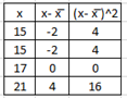 \( \bar{x} = 17 \)
\(s =\sqrt{\frac{ 4 + 4 + 0 + 16}{3}} = \sqrt{8} = 2.8 \)
Ex2. Find range, standard deviation of the following data : 5, 6, 3, 2, 6, 8, 10, 12, 17
Use Statdisk, enter data in column 1, Data/Explore Data/Descriptive Statistics, Select column 1,
Sample standard deviation = 4.72 (rounded)
Range = 15
Ex 3. Find standard deviation of Grouped data.
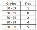 Use the same procedure as finding Grouped mean. Use Statdisk – Frequency Table Generator and Descriptive Statistics.
s = 12.06
3) Inter-quartile-Range
IQR: Q3 – Q1 = middle 50% range of data. IQR is resistance to extreme values.
Ex1. Find Range, Standard Deviation and IQR for
dataset A: 5, 6, 3, 2, 6, 8, 10, 12, 17
dataset B: 5, 6, 3, 2, 6, 8, 10, 12, 17, 60
Range SD IQR
Dataset A: 15 4.7 5
Dataset B: 58 17.1 7
IQR is not influenced by one extreme data.
Other measures related to measure of variation.
1) Population Standard deviation ( σ)
\(\sigma =\sqrt{ \frac{\sum{(x - \mu)^2}}{ N} } \) , where N = population size and x are data from population
Find Population standard deviation online:
https://www.socscistatistics.com/descriptive/variance/default.aspx
2) Variances:
Population variance: \(\sigma ^2 = \frac{\sum{(x - \mu)^2}}{ N} \)
Sample variance: \( s^2 \)
Variances are used in statistical analysis.
Relative standing and Z-score.
Standard deviation is used to describe how far away a value is from the mean.
Sample data = mean + (# of stdev) * stdev.
When comparing values from different dataset, it is best to compare how each value is from their respective mean. The number of standard deviation is a measure of relative standing.
z-score is the number of standard deviations a data value is from the mean.
\( z = \frac{ x - \mu}{\sigma} \) for population data.
\( z = \frac{x - \bar{x}}{s} \) for sample data.
Round-off rule: round to 2 decimal places.
Properties of z-score:
a) z-score tells how many standard deviations a value is from the mean. Negative means below the mean. Positive means above the mean.0
b) z-score has no units.
Ex1:
A student’s English score is 83 when mean = 80 with sd = 10. The student’s History score is 75 when class mean is 72 with sd= 7.
Is the score better in English or History?
English z-score = \( \frac{83-80}{10} = 0.3 \)
History z-score = \( \frac{75-72}{7} = 0.43 \)
The student score less than 1 standard deviation from the mean but since 0.43 > 0.30, hence the student scores better in History.
Ex2.
Ages of 20 fifth graders are given below:
9; 9.5; 9.5; 10; 10; 10; 10; 10.5; 10.5; 10.5; 10.5; 11; 11; 11; 11; 11; 11; 11.5; 11.5; 11.5;
a) Find the mean and standard deviation of ages.
Use statdisk/data/Explore Data/Select data column/Evaluate
mean = 10.5, sd = 0.7
b) What age is one standard deviation above the mean?
10.5 + 1(0.7) = 11.2
c) What age is two standard deviation below the mean?
10.5 - 2(0.7) = 9.1
d) How many data are two standard deviation below the mean or two standard deviation above the mean?
below 2 SD: 10.5 - 2(0.7) = 9.1 or above ; above 2 SD: 10.5 + 2(0.7) = 11.9
one data 9 is below 9.1 and no data are above 11.9.
Ex3.
Measurements of diameter of a bottle cap manufactured in a factory are collected, what situation is best? Explain.
a) High standard deviation.
b) Low standard deviation.
Low standard deviation is better because values will be more consistent and close to the one needed to use for bottle cap.
Ex4. The following histogram show distribution of measurement of diameters of bottle cap from two production line.
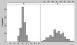
Which histogram left or right one represents sample with low standard deviation? Explain.
The one at the left represent low standard deviation because data are not spread out.