Ch 2.3 and 2.4 Percentile, Boxplot and Outliers
- Page ID
- 15882
\( \newcommand{\vecs}[1]{\overset { \scriptstyle \rightharpoonup} {\mathbf{#1}} } \)
\( \newcommand{\vecd}[1]{\overset{-\!-\!\rightharpoonup}{\vphantom{a}\smash {#1}}} \)
\( \newcommand{\dsum}{\displaystyle\sum\limits} \)
\( \newcommand{\dint}{\displaystyle\int\limits} \)
\( \newcommand{\dlim}{\displaystyle\lim\limits} \)
\( \newcommand{\id}{\mathrm{id}}\) \( \newcommand{\Span}{\mathrm{span}}\)
( \newcommand{\kernel}{\mathrm{null}\,}\) \( \newcommand{\range}{\mathrm{range}\,}\)
\( \newcommand{\RealPart}{\mathrm{Re}}\) \( \newcommand{\ImaginaryPart}{\mathrm{Im}}\)
\( \newcommand{\Argument}{\mathrm{Arg}}\) \( \newcommand{\norm}[1]{\| #1 \|}\)
\( \newcommand{\inner}[2]{\langle #1, #2 \rangle}\)
\( \newcommand{\Span}{\mathrm{span}}\)
\( \newcommand{\id}{\mathrm{id}}\)
\( \newcommand{\Span}{\mathrm{span}}\)
\( \newcommand{\kernel}{\mathrm{null}\,}\)
\( \newcommand{\range}{\mathrm{range}\,}\)
\( \newcommand{\RealPart}{\mathrm{Re}}\)
\( \newcommand{\ImaginaryPart}{\mathrm{Im}}\)
\( \newcommand{\Argument}{\mathrm{Arg}}\)
\( \newcommand{\norm}[1]{\| #1 \|}\)
\( \newcommand{\inner}[2]{\langle #1, #2 \rangle}\)
\( \newcommand{\Span}{\mathrm{span}}\) \( \newcommand{\AA}{\unicode[.8,0]{x212B}}\)
\( \newcommand{\vectorA}[1]{\vec{#1}} % arrow\)
\( \newcommand{\vectorAt}[1]{\vec{\text{#1}}} % arrow\)
\( \newcommand{\vectorB}[1]{\overset { \scriptstyle \rightharpoonup} {\mathbf{#1}} } \)
\( \newcommand{\vectorC}[1]{\textbf{#1}} \)
\( \newcommand{\vectorD}[1]{\overrightarrow{#1}} \)
\( \newcommand{\vectorDt}[1]{\overrightarrow{\text{#1}}} \)
\( \newcommand{\vectE}[1]{\overset{-\!-\!\rightharpoonup}{\vphantom{a}\smash{\mathbf {#1}}}} \)
\( \newcommand{\vecs}[1]{\overset { \scriptstyle \rightharpoonup} {\mathbf{#1}} } \)
\(\newcommand{\longvect}{\overrightarrow}\)
\( \newcommand{\vecd}[1]{\overset{-\!-\!\rightharpoonup}{\vphantom{a}\smash {#1}}} \)
\(\newcommand{\avec}{\mathbf a}\) \(\newcommand{\bvec}{\mathbf b}\) \(\newcommand{\cvec}{\mathbf c}\) \(\newcommand{\dvec}{\mathbf d}\) \(\newcommand{\dtil}{\widetilde{\mathbf d}}\) \(\newcommand{\evec}{\mathbf e}\) \(\newcommand{\fvec}{\mathbf f}\) \(\newcommand{\nvec}{\mathbf n}\) \(\newcommand{\pvec}{\mathbf p}\) \(\newcommand{\qvec}{\mathbf q}\) \(\newcommand{\svec}{\mathbf s}\) \(\newcommand{\tvec}{\mathbf t}\) \(\newcommand{\uvec}{\mathbf u}\) \(\newcommand{\vvec}{\mathbf v}\) \(\newcommand{\wvec}{\mathbf w}\) \(\newcommand{\xvec}{\mathbf x}\) \(\newcommand{\yvec}{\mathbf y}\) \(\newcommand{\zvec}{\mathbf z}\) \(\newcommand{\rvec}{\mathbf r}\) \(\newcommand{\mvec}{\mathbf m}\) \(\newcommand{\zerovec}{\mathbf 0}\) \(\newcommand{\onevec}{\mathbf 1}\) \(\newcommand{\real}{\mathbb R}\) \(\newcommand{\twovec}[2]{\left[\begin{array}{r}#1 \\ #2 \end{array}\right]}\) \(\newcommand{\ctwovec}[2]{\left[\begin{array}{c}#1 \\ #2 \end{array}\right]}\) \(\newcommand{\threevec}[3]{\left[\begin{array}{r}#1 \\ #2 \\ #3 \end{array}\right]}\) \(\newcommand{\cthreevec}[3]{\left[\begin{array}{c}#1 \\ #2 \\ #3 \end{array}\right]}\) \(\newcommand{\fourvec}[4]{\left[\begin{array}{r}#1 \\ #2 \\ #3 \\ #4 \end{array}\right]}\) \(\newcommand{\cfourvec}[4]{\left[\begin{array}{c}#1 \\ #2 \\ #3 \\ #4 \end{array}\right]}\) \(\newcommand{\fivevec}[5]{\left[\begin{array}{r}#1 \\ #2 \\ #3 \\ #4 \\ #5 \\ \end{array}\right]}\) \(\newcommand{\cfivevec}[5]{\left[\begin{array}{c}#1 \\ #2 \\ #3 \\ #4 \\ #5 \\ \end{array}\right]}\) \(\newcommand{\mattwo}[4]{\left[\begin{array}{rr}#1 \amp #2 \\ #3 \amp #4 \\ \end{array}\right]}\) \(\newcommand{\laspan}[1]{\text{Span}\{#1\}}\) \(\newcommand{\bcal}{\cal B}\) \(\newcommand{\ccal}{\cal C}\) \(\newcommand{\scal}{\cal S}\) \(\newcommand{\wcal}{\cal W}\) \(\newcommand{\ecal}{\cal E}\) \(\newcommand{\coords}[2]{\left\{#1\right\}_{#2}}\) \(\newcommand{\gray}[1]{\color{gray}{#1}}\) \(\newcommand{\lgray}[1]{\color{lightgray}{#1}}\) \(\newcommand{\rank}{\operatorname{rank}}\) \(\newcommand{\row}{\text{Row}}\) \(\newcommand{\col}{\text{Col}}\) \(\renewcommand{\row}{\text{Row}}\) \(\newcommand{\nul}{\text{Nul}}\) \(\newcommand{\var}{\text{Var}}\) \(\newcommand{\corr}{\text{corr}}\) \(\newcommand{\len}[1]{\left|#1\right|}\) \(\newcommand{\bbar}{\overline{\bvec}}\) \(\newcommand{\bhat}{\widehat{\bvec}}\) \(\newcommand{\bperp}{\bvec^\perp}\) \(\newcommand{\xhat}{\widehat{\xvec}}\) \(\newcommand{\vhat}{\widehat{\vvec}}\) \(\newcommand{\uhat}{\widehat{\uvec}}\) \(\newcommand{\what}{\widehat{\wvec}}\) \(\newcommand{\Sighat}{\widehat{\Sigma}}\) \(\newcommand{\lt}{<}\) \(\newcommand{\gt}{>}\) \(\newcommand{\amp}{&}\) \(\definecolor{fillinmathshade}{gray}{0.9}\)Percentile and Quartiles
Percentile: are measures of location. Denoted by P1, P2, … P99 which divide a set of data into 100 groups with about 1% of the values in each group.
If x is at 90th percentile, means 90% of all data are less than x. Note, percentile is not the same as percentage.
Quartiles: (Q1, Q2, Q3 )
Quartiles are measures of location, which divide a set of data into four groups with about 25% of the values in each group.
Q1 – First quartile or P25. It separates the bottom 25% of value from the top 75%.
Q2 - Second quartile or P50 or median. It separates the bottom 50% of values from the top 50%.
Q3 – Third quartile or P75. It separates the bottom 75% of values from the top 25%.
Five-number-summary, IQR and Boxplot:
Five-number-summary are:
Mininum, Q1, Median, Q3 and Maximum divides the data into four groups of 25% each.
IQR = Q3 – Q1 (Inter-quantile Range)
The interquartile range (IQR) is a number that indicates the spread of the middle half or the middle 50% of the data. It is the difference between the third quartile (Q3) and the first quartile (Q1).
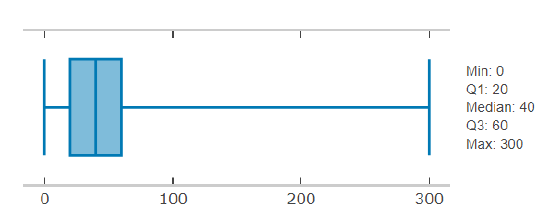
A boxplot shows graphical image of concentration of data. A boxplot is constructed using 5-number summary with Q1, median and Q3 in a box containing 50% of all data. It gives good distribution of data in 25%, 50% and 75%.
- Maximum and Minimum values are extended as whiskers at the two ends of the box.
Find 5-number-summary and boxplot by Statdisk
- Enter data in a column in Statdisk.
- Select Data, Explore data, descriptive statistic, select column and Click evaluate.
Ex1. The time(in min.) a sample of 15 student spent on exercising daily is given:
0, 40, 60, 30, 60, 10, 46, 30, 300, 90, 30, 120, 60, 0, 20
a) Find the 5-number summary and sketch a boxplot.
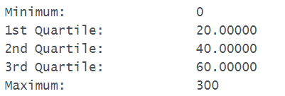
Use statdisk, data/explore data/select column data/evaluate, five number summary and boxplot will show.


b) What percent of student exercise from 0 to 60 min?
Because 60 is Q3, so 75% of all student exercise from 0 to 60 min.
c) What percent of student exercise between 20 to 60 min?
Because 20 is Q1, 60 is Q3, so 50% of all students exercise from 20 to 60 min.
Answer: Use Statdisk:
a) Min = 0, Q1=20, Med=40, Q3=60, Max = 300

b) Since Q3 = 60, hence 75% of students exercise from 0 to 60 min.
c) Since Q1 = 20 and Q3=60, Hence 50% of students exercise from 20 to 60 min.
Outliers and IQR
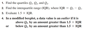
IQR is used to determine potential outliers.

Ex1. If Q1 = 34, Q3 = 70, find the lower fence and upper fence for an outlier.
IQR = 70 - 34 = 36
lower fence is 34 - 1.5(36) = -20, upper fence = 70 + 1.5(36) = 124
Value between -20 and 124 are not outliers, values outside the range are outliers.
A potential outlier is a data point that is significantly different from the other data points. These special data points may be errors or some kind of abnormality or they may be a key to understanding the data.
C) Modified boxplot and outliers:
A modified boxplot can be graphed to show outliers without calculating IQR and applying the Q1-1.5IQR, Q3+1.5IQR. Outliers are shown as markers in the boxplot.
- use Statdisk, click data , Boxplot,
- Select the column of data, click modified boxplot. The outlier will be shown as marker at the lowest or highest end of the boxplot.
- If there are no markers, there is no outliers in the dataset.
- To find the values of the outlier, sort the data. The outliers will be at the top and end of the sorted data.
Ex2. Determine if outliers exist in the exercise time from 15 students.
0, 40, 60, 30, 60, 10, 46, 30, 300, 90, 30, 120, 60, 0, 20
By calculation:
Since Q1 = 20, Q3 = 60, So IQR = 60 – 20 = 40
Lower fence = Q1 – 1.5(IQR) = 20 – 1.5(40) = -40
upper fence = Q3 + 1.5(IQR) = 60 + 1.5(40) = 120
Values lower than -40 and higher than 120 is an outlier. So the value 300 is an outlier.
Graph a modified boxplot to identify outliers.
Use Statdisk, Data/Boxplot/select Modified boxplot.

There is one outlier in the high end of the data. To find the outlier, sort the data and locate the highest value.
Use Statdisk, Sort, one column, select the column containing the data. The last data (300) is the outlier.

