Ch 6.1 Standard Normal Distribution

Ch 6.1 Standard Normal distribution

Normal Density Curve

A random variable X has a distribution with a graph that is symmetric and bell-shaped, and it can be described by the equation given by

\( y = \frac{e^{\frac{-1}{2}\cdot {(\frac{x-\mu}{\sigma})}^2}}{\sigma \sqrt{2 \pi}} \) , then it has a “Normal distribution”

Normal Density Curve:

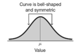
Note: the distribution is determined by μ  and  σ.

 

 

 

Z-score

Z-score of x =  \( \frac{x-\mu}{\sigma} \) is the standardized value of x.

z-score tells the number of standard deviation X is above or below the mean. Positive z implies X is above the mean, negative z implies X is below the mean.

 

A) Standard Normal

  (also known as z distribution) is a normal distribution with parameters:

Mean μ = 0 and standard deviation σ = 1.

 The total area under its density curve is equal to 1.

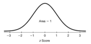
Properties of standard normal (z-normal):

- area left of z of 0 = 0.5

- area right of z of 0 = 0.5

- area left of z =  area right of  - z

- area right of z = 1 – area left of z

 

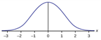
B) Empirical Rule (68-95-99.7)

If X is normally distributed, 68% are within 1 sd from the mean. 95% are within 2 sd from the mean, 99.7% are within 3 sd from the mean.

P( Z-score between -1 and 1 ) = 68%

P( Z-score between -2 and 2 ) = 95%

P( Z-score between -3 and 3 ) = 99.7%

Ex1.  Weight of a certain type of dog is normally distributed with mean = 18 lb. and standard deviation of 2 lb.

   write the marking of mean, mean - 1sd, mean - 2sd, mean + sd, mean + 2d on a number line.

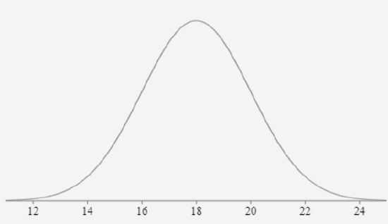
a) What is the z-score of 14lb and 22 lb? What is the probability that a dog weighs between 14 lb and 22lb?

14 and 22 are 2 sd from the mean, so according to the Empirical rule, the probability is 95%.

b) What is the z-score of 20lb and 16lb? What is the probability that a dog weighs between 16lb and 20 lb?

16 and 20 are 1 sd from the mean, so according to the Empirical rule, the probability is 68%.

c) What is the z-score of 24 lb and 12 lb? What is the probability that a dog weigh between 12 lb and 24lb?

                                                                     24 is 3 sd above the mean, so z-score of 24 lb is 3.

                                                                     12 is 3 sd below the mean, so z-score of 12 lb is -3.

C) Probability of z-score in standard normal

 Use online Normal distribution calculator

http://onlinestatbook.com/2/calculators/normal_dist.html

Specify mean μ =0  standard deviation &sigma&

-For left area or P(x < a) click below

-For right area or P(x > a) click above

-For area between two values a and b P( a < x < b), click between

-For area outside of a and b, P(x < a or x > b), click outside

-Click “Recalculate”

 

Ex1: Find probability that z is between -1.8  and 1.8. Sketch the area.

 

Use online Normal calculator Mean = 0, SD = 1

Click between, enter -1.8, 1.8

Recalculate: P( -1.8 < z < 1.8 ) = 0.9281

 

Ex2. Find the probability that z is less than 0.44. Sketch the area.

 

Use online Normal calculator μ =0 , SD=1

Click below , enter 0.44

Recalculate: P( z < 0.44 ) = 0.67

 

 Ex3. Find the probability that z is greater than 1.8.  Sketch the area.

 

Use online Normal calculator μ =0 , SD=1

Click above , enter 1.8

Recalculate: P( z >1.8) = 0.0359

 

Ex 4. Find the probability that z is less than – 1.2. Sketch the area.

Use online Normal calculator μ =0 , SD=1

Click below , enter -1.2

Recalculate: P( z < -1.2) = 0.1151

D) Find percentile of a z-score

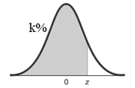k Percentile corresponds to a value that is higher thank% of all values. Or k% of data are less than the k percentile value. This corresponds to left area of k%.

 

 

Ex5. What percentile is the z-score 2.2?

Use online Normal calculator Mean =0 , SD=1

Percentile is referring to 2.2 or less. Click below , enter 2.2

Recalculate: P( z < 2.2) = 0.9861 = 98.6%

Round to whole percent = 99th percentile

 

Ex 6. What percentile is the z-score -1.35

Use online Normal calculator μ =0 , σ=1

Click below , enter -1.35

Recalculate: P( z < -1.35) = 0.0885 = 8.9%

Round to whole percent. 9th percentile

 

E) Find z-score given area or percentile.

 Online Inverse Normal calculator is use to find the z-score that is the cut-off for the left area, right area or percentile.

http://onlinestatbook.com/2/calculators/inverse_normal_dist.html

Specify area, mean= 0 and SD= 1

Select if area is below, above, between or outside.

Click “Recalculate”

 

Ex1. Find the z-score that corresponds to bottom 10% of all values.

Use Inverse Normal Calculator. Convert 10% to  0.1.

Specify area = 0.1, Mean = 0, sd =1,

Click below.

Recalculate.   P( z < __-1.28_____ ) = 0.1,   cut-off z = -1.28

 

Ex2.  Find the cutoff for top 20%.

Use Inverse Normal Calculator. Convert 20% to  0.2.

Specify area = 0.2

Mean = 0, sd =1,

Click above  ( for top percent). Recalculate.

P( z >  __0.842______) = 0.2  z-cutoff = 0.84

 

Ex3. Find P₉₁ , 91th percentile of all z.

Use Inverse Normal calculator.

Specify area = 0.91

Mean = 0, sd =1,

Click below. Recalculate.

P( z <  __1.341______) = 0.91  91th percentile of all z = 1.34.

 

Ex4. Find P_15, 15^th percentile of all z.

Convert 15% = 0.15. Use Inverse Normal calculator.

Specify area = 0.15, Mean = 0, sd =1,

Click below. Recalculate

 P( z <  _-1.036_______) = 0.15  15th percentile = -1.04

 

F) Find Critical value Z_α

α = significant level. The probability of unlikely, default is 0.05 if not specify.

Critical value z_α : the positive z-value that separates significantly high values of  z with non-significant z.

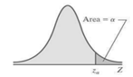Note: Significantly low critical value = - z_α 

 

 

 

To find z_α:  Use Inverse Normal calculator

Specify area = α, Mean = 0, sd =1,

Click above. Recalculate.

 

Ex1. Given α = 0.02, Find the critical value Z_0.02. 

Use Inverse Normal calculator

Specify area = 0.02, Mean = 0, sd =1,

Click above. Recalculate.

Z_0.02 = 2.054

 

Ex2. Given α = 0.06, find the critical value Z_0.06

Use Inverse Normal calculator

Specify area = 0.06, Mean = 0, sd =1,

Click above. Recalculate.

Z_0.06 = 1.555