6.4: Applications of Finding Normal Probabilities

Last updated
Save as PDF

Page ID: 26072

\( \newcommand{\vecs}[1]{\overset { \scriptstyle \rightharpoonup} {\mathbf{#1}} } \) \( \newcommand{\vecd}[1]{\overset{-\!-\!\rightharpoonup}{\vphantom{a}\smash {#1}}} \)\(\newcommand{\id}{\mathrm{id}}\) \( \newcommand{\Span}{\mathrm{span}}\) \( \newcommand{\kernel}{\mathrm{null}\,}\) \( \newcommand{\range}{\mathrm{range}\,}\) \( \newcommand{\RealPart}{\mathrm{Re}}\) \( \newcommand{\ImaginaryPart}{\mathrm{Im}}\) \( \newcommand{\Argument}{\mathrm{Arg}}\) \( \newcommand{\norm}[1]{\| #1 \|}\) \( \newcommand{\inner}[2]{\langle #1, #2 \rangle}\) \( \newcommand{\Span}{\mathrm{span}}\) \(\newcommand{\id}{\mathrm{id}}\) \( \newcommand{\Span}{\mathrm{span}}\) \( \newcommand{\kernel}{\mathrm{null}\,}\) \( \newcommand{\range}{\mathrm{range}\,}\) \( \newcommand{\RealPart}{\mathrm{Re}}\) \( \newcommand{\ImaginaryPart}{\mathrm{Im}}\) \( \newcommand{\Argument}{\mathrm{Arg}}\) \( \newcommand{\norm}[1]{\| #1 \|}\) \( \newcommand{\inner}[2]{\langle #1, #2 \rangle}\) \( \newcommand{\Span}{\mathrm{span}}\)\(\newcommand{\AA}{\unicode[.8,0]{x212B}}\)

The shaded area in the following graph indicates the area to the left of \(x\). This area is represented by the probability \(P(X < x)\). Normal tables, computers, and calculators provide or calculate the probability \(P(X < x)\).

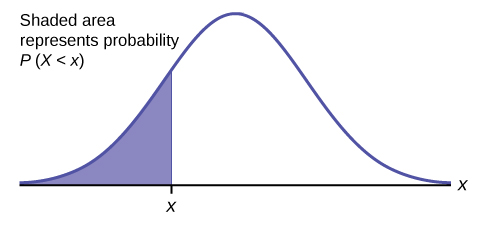
The area to the right is then \(P(X > x) = 1 – P(X < x)\). Remember, \(P(X < x) =\) Area to the left of the vertical line through \(x\). \(P(X > x) = 1 – P(X < x) =\) Area to the right of the vertical line through \(x\). \(P(X < x)\) is the same as \(P(X \leq x)\) and \(P(X > x)\) is the same as \(P(X \geq x)\) for continuous distributions.

Calculations of Probabilities

Probabilities involving normal distributions are usually calculated using technology such as calculators or spreadsheets. The can also be calculated using probability tables provided in [link] without the use of technology. The tables include instructions for how to use them.

Example \(\PageIndex{2}\)

The final exam scores in a statistics class were normally distributed with a mean of 63 and a standard deviation of five.

Find the probability that a randomly selected student scored more than 65 on the exam.
Find the probability that a randomly selected student scored less than 85.
Find the 90^th percentile (that is, find the score \(k\) that has 90% of the scores below k and 10% of the scores above \(k\)).
Find the 70^th percentile (that is, find the score \(k\) such that 70% of scores are below \(k\) and 30% of the scores are above \(k\)).

Answer

a. Let \(X\) = a score on the final exam. \(X \sim N(63, 5)\), where \(\mu = 63\) and \(\sigma = 5\)

Draw a graph.

Then, find \(P(x > 65)\).

\[P(x > 65) = 0.3446\nonumber \]

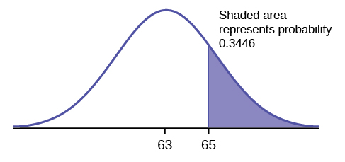
The probability that any student selected at random scores more than 65 is 0.3446.

Example \(\PageIndex{3}\)

A personal computer is used for office work at home, research, communication, personal finances, education, entertainment, social networking, and a myriad of other things. Suppose that the average number of hours a household personal computer is used for entertainment is two hours per day. Assume the times for entertainment are normally distributed and the standard deviation for the times is half an hour.

Find the probability that a household personal computer is used for entertainment between 1.8 and 2.75 hours per day.
Find the maximum number of hours per day that the bottom quartile of households uses a personal computer for entertainment.

Answer

a. Let \(X =\) the amount of time (in hours) a household personal computer is used for entertainment. \(X \sim N(2, 0.5)\) where \(\mu = 2\) and \(\sigma = 0.5\).

Find \(P(1.8 < x < 2.75)\).

The probability for which you are looking is the area between \(x = 1.8\) and \(x = 2.75\). \(P(1.8 < x < 2.75) = 0.5886\)

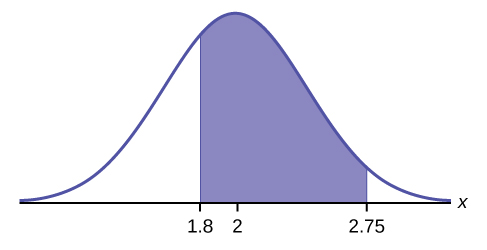
\[\text{normalcdf}(1.8,2.75,2,0.5) = 0.5886\nonumber \]

The probability that a household personal computer is used between 1.8 and 2.75 hours per day for entertainment is 0.5886.

To find the maximum number of hours per day that the bottom quartile of households uses a personal computer for entertainment, find the 25^th percentile, \(k\), where \(P(x < k) = 0.25\).

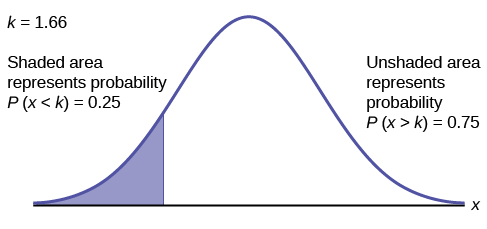
\[\text{invNorm}(0.25,2,0.5) = 1.66\nonumber \]

The maximum number of hours per day that the bottom quartile of households uses a personal computer for entertainment is 1.66 hours.

Example \(\PageIndex{4}\)

There are approximately one billion smartphone users in the world today. In the United States the ages 13 to 55+ of smartphone users approximately follow a normal distribution with approximate mean and standard deviation of 36.9 years and 13.9 years, respectively.

Determine the probability that a random smartphone user in the age range 13 to 55+ is between 23 and 64.7 years old.
Determine the probability that a randomly selected smartphone user in the age range 13 to 55+ is at most 50.8 years old.
Find the 80^th percentile of this distribution, and interpret it in a complete sentence.

Answer

\(\text{normalcdf}(23,64.7,36.9,13.9) = 0.8186\)
\(\text{normalcdf}(-10^{99},50.8,36.9,13.9) = 0.8413\)
\(\text{invNorm}(0.80,36.9,13.9) = 48.6\)

The 80^th percentile is 48.6 years.

80% of the smartphone users in the age range 13 – 55+ are 48.6 years old or less.

Example \(\PageIndex{5}\)

In the United States the ages 13 to 55+ of smartphone users approximately follow a normal distribution with approximate mean and standard deviation of 36.9 years and 13.9 years respectively. Using this information, answer the following questions (round answers to one decimal place).

Calculate the interquartile range (\(IQR\)).
Forty percent of the ages that range from 13 to 55+ are at least what age?

Answer

\[IQR = Q_{3} – Q_{1}\nonumber \]

Calculate \(Q_{3} =\) 75^th percentile and \(Q_{1} =\) 25^th percentile.

Find \(k\) where \(P(x > k) = 0.40\) ("At least" translates to "greater than or equal to.")

\(0.40 =\) the area to the right.

Area to the left \(= 1 – 0.40 = 0.60\).

The area to the left of \(k = 0.60\).

\(\text{invNorm}(0.60,36.9,13.9) = 40.4215\).

\(k = 40.42\).

Forty percent of the smartphone users from 13 to 55+ are at least 40.4 years.

Exercise \(\PageIndex{5}\)

WeBWorK Problems

Query \(\PageIndex{1}\)

Query \(\PageIndex{2}\)

Query \(\PageIndex{3}\)

Query \(\PageIndex{4}\)

Query \(\PageIndex{1}\)

Query \(\PageIndex{4}\)

References

“Naegele’s rule.” Wikipedia. Available online at http://en.Wikipedia.org/wiki/Naegele's_rule (accessed May 14, 2013).
“403: NUMMI.” Chicago Public Media & Ira Glass, 2013. Available online at www.thisamericanlife.org/radi...sode/403/nummi (accessed May 14, 2013).
“Scratch-Off Lottery Ticket Playing Tips.” WinAtTheLottery.com, 2013. Available online at www.winatthelottery.com/publi...partment40.cfm (accessed May 14, 2013).
“Smart Phone Users, By The Numbers.” Visual.ly, 2013. Available online at http://visual.ly/smart-phone-users-numbers (accessed May 14, 2013).
“Facebook Statistics.” Statistics Brain. Available online at http://www.statisticbrain.com/facebo...tics/(accessed May 14, 2013).

Review

The normal distribution, which is continuous, is the most important of all the probability distributions. Its graph is bell-shaped. This bell-shaped curve is used in almost all disciplines. Since it is a continuous distribution, the total area under the curve is one. The parameters of the normal are the mean \(\mu\) and the standard deviation σ. A special normal distribution, called the standard normal distribution is the distribution of z-scores. Its mean is zero, and its standard deviation is one.

Contributors and Attributions

Barbara Illowsky and Susan Dean (De Anza College) with many other contributing authors. Content produced by OpenStax College is licensed under a Creative Commons Attribution License 4.0 license. Download for free at http://cnx.org/contents/30189442-699...b91b9de@18.114.