6.3: The Standard Normal Distribution

Introduction to Normal Distributions

The normal distribution is the most important of all the probability distributions. It is widely used and even more widely abused. Its graph is bell-shaped. You see the bell curve in almost all disciplines. Some of these include psychology, business, economics, the sciences, nursing, and, of course, mathematics. Some of your instructors may use the normal distribution to help determine your grade. Most IQ scores are normally distributed. Often real-estate prices fit a normal distribution. The normal distribution is extremely important, but it cannot be applied to everything in the real world.

In the remainder of this chapter, you will study the normal distributions and applications associated with them. A normal distribution has two parameters (two numerical descriptive measures), the mean (\(\mu\)) and the standard deviation (\(\sigma\)). If \(X\) is a quantity to be measured that has a normal distribution with mean (\(\mu\)) and standard deviation (\(\sigma\)), we designate this by writing

\[f(x) = \dfrac{1}{\sigma \cdot \sqrt{2 \cdot \pi}} \cdot e^{\left(-\dfrac{1}{2}\right) \cdot \left(\dfrac{x-\mu}{\sigma}\right)^{2}}\]

The probability density function is a rather complicated function. Do not memorize it. It is not necessary.

The cumulative distribution function is \(P(X < x)\). It is calculated either by a calculator or a computer, or it is looked up in a table. Technology has made the tables virtually obsolete. For that reason, as well as the fact that there are various table formats, we are not including table instructions.

Figure \(\PageIndex{2}\): The standard normal distribution

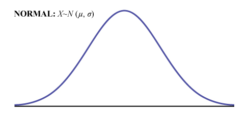
The curve is symmetrical about a vertical line drawn through the mean, \(\mu\). In theory, the mean is the same as the median, because the graph is symmetric about \(\mu\). As the notation indicates, the normal distribution depends only on the mean and the standard deviation. Since the area under the curve must equal one, a change in the standard deviation, \(\sigma\), causes a change in the shape of the curve; the curve becomes fatter or skinnier depending on \(\sigma\). A change in \(\mu\) causes the graph to shift to the left or right. This means there are an infinite number of normal probability distributions. One of special interest is called the standard normal distribution.

COLLABORATIVE CLASSROOM ACTIVITY

Your instructor will record the heights of both men and women in your class, separately. Draw histograms of your data. Then draw a smooth curve through each histogram. Is each curve somewhat bell-shaped? Do you think that if you had recorded 200 data values for men and 200 for women that the curves would look bell-shaped? Calculate the mean for each data set. Write the means on the x-axis of the appropriate graph below the peak. Shade the approximate area that represents the probability that one randomly chosen male is taller than 72 inches. Shade the approximate area that represents the probability that one randomly chosen female is shorter than 60 inches. If the total area under each curve is one, does either probability appear to be more than 0.5?

Formula Review

• \(X \sim N(\mu, \sigma)\)
• \(\mu =\) the mean \(\sigma =\) the standard deviation

Z-Scores

The standard normal distribution is a normal distribution of standardized values called z-scores. A z-score is measured in units of the standard deviation.

Definition: Z-Score

If \(X\) is a normally distributed random variable and \(X \sim N(\mu, \sigma)\), then the z-score is:

\[z = \frac{x - \mu}{\sigma}\]

The z-score tells you how many standard deviations the value \(x\) is above (to the right of) or below (to the left of) the mean, \(\mu\). Values of \(x\) that are larger than the mean have positive \(z\)-scores, and values of \(x\) that are smaller than the mean have negative \(z\)-scores. If \(x\) equals the mean, then \(x\) has a \(z\)-score of zero. For example, if the mean of a normal distribution is five and the standard deviation is two, the value 11 is three standard deviations above (or to the right of) the mean. The calculation is as follows:

\[ \begin{align*} x &= \mu + (z)(\sigma) \\[5pt] &= 5 + (3)(2) = 11 \end{align*}\]

The z-score is three.

Since the mean for the standard normal distribution is zero and the standard deviation is one, then the transformation in Equation \ref{zscore} produces the distribution \(Z \sim N(0, 1)\). The value \(x\) comes from a normal distribution with mean \(\mu\) and standard deviation \(\sigma\).

A z-score is measured in units of the standard deviation.

Example \(\PageIndex{1}\)

Suppose \(X \sim N(5, 6)\). This says that \(x\) is a normally distributed random variable with mean \(\mu = 5\) and standard deviation \(\sigma = 6\). Suppose \(x = 17\). Then (via Equation \ref{zscore}):

\[z = \dfrac{x-\mu}{\sigma} = \dfrac{17-5}{6} = 2 \nonumber\]

This means that \(x = 17\) is two standard deviations (2\(\sigma\)) above or to the right of the mean \(\mu = 5\). The standard deviation is \(\sigma = 6\).

Notice that: \(5 + (2)(6) = 17\) (The pattern is \(\mu + z \sigma = x\))

Now suppose \(x = 1\). Then:

\[z = \dfrac{x-\mu}{\sigma} = \dfrac{1-5}{6} = -0.67 \nonumber\]

(rounded to two decimal places)

This means that \(x = 1\) is \(0.67\) standard deviations (\(–0.67\sigma\)) below or to the left of the mean \(\mu = 5\). Notice that: \(5 + (–0.67)(6)\) is approximately equal to one (This has the pattern \(\mu + (–0.67)\sigma = 1\))

Summarizing, when \(z\) is positive, \(x\) is above or to the right of \(\mu\) and when \(z\) is negative, \(x\) is to the left of or below \(\mu\). Or, when \(z\) is positive, \(x\) is greater than \(\mu\), and when \(z\) is negative \(x\) is less than \(\mu\).

Example \(\PageIndex{2}\)

Some doctors believe that a person can lose five pounds, on the average, in a month by reducing his or her fat intake and by exercising consistently. Suppose weight loss has a normal distribution. Let \(X =\) the amount of weight lost(in pounds) by a person in a month. Use a standard deviation of two pounds. \(X \sim N(5, 2)\). Fill in the blanks.

1. Suppose a person lost ten pounds in a month. The \(z\)-score when \(x = 10\) pounds is \(x = 2.5\) (verify). This \(z\)-score tells you that \(x = 10\) is ________ standard deviations to the ________ (right or left) of the mean _____ (What is the mean?).
2. Suppose a person gained three pounds (a negative weight loss). Then \(z =\) __________. This \(z\)-score tells you that \(x = -3\) is ________ standard deviations to the __________ (right or left) of the mean.

Answers

a. This \(z\)-score tells you that \(x = 10\) is 2.5 standard deviations to the right of the mean five.

b. Suppose the random variables \(X\) and \(Y\) have the following normal distributions: \(X \sim N(5, 6)\) and \(Y \sim N(2, 1)\). If \(x = 17\), then \(z = 2\). (This was previously shown.) If \(y = 4\), what is \(z\)?

\[z = \dfrac{y-\mu}{\sigma} = \dfrac{4-2}{1} = 2 \nonumber\]

where \(\mu = 2\) and \(\sigma = 1\).

The \(z\)-score for \(y = 4\) is \(z = 2\). This means that four is \(z = 2\) standard deviations to the right of the mean. Therefore, \(x = 17\) and \(y = 4\) are both two (of their own) standard deviations to the right of their respective means.

The z-score allows us to compare data that are scaled differently. To understand the concept, suppose \(X \sim N(5, 6)\) represents weight gains for one group of people who are trying to gain weight in a six week period and \(Y \sim N(2, 1)\) measures the same weight gain for a second group of people. A negative weight gain would be a weight loss. Since \(x = 17\) and \(y = 4\) are each two standard deviations to the right of their means, they represent the same, standardized weight gain relative to their means.

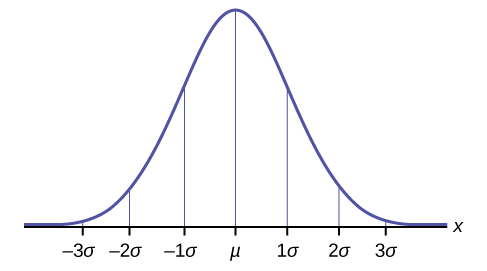
The Empirical Rule

If \(X\) is a random variable and has a normal distribution with mean \(\mu\) and standard deviation \(\sigma\), then the Empirical Rule says the following:

• About 68% of the \(x\) values lie between –1\(\sigma\) and +1\(\sigma\) of the mean \(\mu\) (within one standard deviation of the mean).
• About 95% of the \(x\) values lie between –2\(\sigma\) and +2\(\sigma\) of the mean \(\mu\) (within two standard deviations of the mean).
• About 99.7% of the \(x\) values lie between –3\(\sigma\) and +3\(\sigma\) of the mean \(\mu\) (within three standard deviations of the mean). Notice that almost all the \(x\) values lie within three standard deviations of the mean.
• The \(z\)-scores for +1\(\sigma\) and –1\(\sigma\) are +1 and –1, respectively.
• The \(z\)-scores for +2\(\sigma\) and –2\(\sigma\) are +2 and –2, respectively.
• The \(z\)-scores for +3\(\sigma\) and –3\(\sigma\) are +3 and –3 respectively.

The empirical rule is also known as the 68-95-99.7 rule.

Figure \(\PageIndex{1}\)

Example \(\PageIndex{3}\)

The mean height of 15 to 18-year-old males from Chile from 2009 to 2010 was 170 cm with a standard deviation of 6.28 cm. Male heights are known to follow a normal distribution. Let \(X =\) the height of a 15 to 18-year-old male from Chile in 2009 to 2010. Then \(X \sim N(170, 6.28)\).

1. Suppose a 15 to 18-year-old male from Chile was 168 cm tall from 2009 to 2010. The \(z\)-score when \(x = 168\) cm is \(z =\) _______. This \(z\)-score tells you that \(x = 168\) is ________ standard deviations to the ________ (right or left) of the mean _____ (What is the mean?).
2. Suppose that the height of a 15 to 18-year-old male from Chile from 2009 to 2010 has a \(z\)-score of \(z = 1.27\). What is the male’s height? The \(z\)-score (\(z = 1.27\)) tells you that the male’s height is ________ standard deviations to the __________ (right or left) of the mean.

Answers

1. –0.32, 0.32, left, 170
2. 177.98, 1.27, right 

Example \(\PageIndex{4}\)

From 1984 to 1985, the mean height of 15 to 18-year-old males from Chile was 172.36 cm, and the standard deviation was 6.34 cm. Let \(Y =\) the height of 15 to 18-year-old males from 1984 to 1985. Then \(Y \sim N(172.36, 6.34)\).

The mean height of 15 to 18-year-old males from Chile from 2009 to 2010 was 170 cm with a standard deviation of 6.28 cm. Male heights are known to follow a normal distribution. Let \(X =\) the height of a 15 to 18-year-old male from Chile in 2009 to 2010. Then \(X \sim N(170, 6.28)\).

Find the z-scores for \(x = 160.58\) cm and \(y = 162.85\) cm. Interpret each \(z\)-score. What can you say about \(x = 160.58\) cm and \(y = 162.85\) cm?

Answer

• The \(z\)-score (Equation \ref{zscore}) for \(x = 160.58\) is \(z = –1.5\).
• The \(z\)-score for \(y = 162.85\) is \(z = –1.5\).

Both \(x = 160.58\) and \(y = 162.85\) deviate the same number of standard deviations from their respective means and in the same direction.

Example \(\PageIndex{5}\)

Suppose x has a normal distribution with mean 50 and standard deviation 6.

• About 68% of the x values lie within one standard deviation of the mean. Therefore, about 68% of the x values lie between –1σ = (–1)(6) = –6 and 1σ = (1)(6) = 6 of the mean 50. The values 50 – 6 = 44 and 50 + 6 = 56 are within one standard deviation from the mean 50. The z-scores are –1 and +1 for 44 and 56, respectively.
• About 95% of the x values lie within two standard deviations of the mean. Therefore, about 95% of the x values lie between –2σ = (–2)(6) = –12 and 2σ = (2)(6) = 12. The values 50 – 12 = 38 and 50 + 12 = 62 are within two standard deviations from the mean 50. The z-scores are –2 and +2 for 38 and 62, respectively.
• About 99.7% of the x values lie within three standard deviations of the mean. Therefore, about 99.7% of the x values lie between –3σ = (–3)(6) = –18 and 3σ = (3)(6) = 18 from the mean 50. The values 50 – 18 = 32 and 50 + 18 = 68 are within three standard deviations of the mean 50. The z-scores are –3 and +3 for 32 and 68, respectively.

Example \(\PageIndex{6}\)

From 1984 to 1985, the mean height of 15 to 18-year-old males from Chile was 172.36 cm, and the standard deviation was 6.34 cm. Let \(Y =\) the height of 15 to 18-year-old males in 1984 to 1985. Then \(Y \sim N(172.36, 6.34)\).

1. About 68% of the \(y\) values lie between what two values? These values are ________________. The \(z\)-scores are ________________, respectively.
2. About 95% of the \(y\) values lie between what two values? These values are ________________. The \(z\)-scores are ________________ respectively.
3. About 99.7% of the \(y\) values lie between what two values? These values are ________________. The \(z\)-scores are ________________, respectively.

Answer

1. About 68% of the values lie between 166.02 and 178.7. The \(z\)-scores are –1 and 1.
2. About 95% of the values lie between 159.68 and 185.04. The \(z\)-scores are –2 and 2.
3. About 99.7% of the values lie between 153.34 and 191.38. The \(z\)-scores are –3 and 3.

Summary

A \(z\)-score is a standardized value. Its distribution is the standard normal, \(Z \sim N(0,1)\). The mean of the \(z\)-scores is zero and the standard deviation is one. If \(y\) is the z-score for a value \(x\) from the normal distribution \(N(\mu, \sigma)\) then \(z\) tells you how many standard deviations \(x\) is above (greater than) or below (less than) \(\mu\).

Formula Review

\(Z \sim N(0, 1)\)

\(z = a\) standardized value (\(z\)-score)

mean = 0; standard deviation = 1

To find the \(K\)^th percentile of \(X\) when the \(z\)-scores is known:

\(k = \mu + (z)\sigma\)

\(z\)-score: \(z = \dfrac{x-\mu}{\sigma}\)

\(Z =\) the random variable for z-scores

\(Z \sim N(0, 1)\)

WebWork Problems

Query \(\PageIndex{1}\)

Query \(\PageIndex{2}\)

Query \(\PageIndex{3}\)

Query \(\PageIndex{4}\)

Query \(\PageIndex{5}\)

Query \(\PageIndex{6}\)

Glossary

Standard Normal Distribution

a continuous random variable (RV) \(X \sim N(0, 1)\); when \(X\) follows the standard normal distribution, it is often noted as \(Z \sim N(0, 1)\.

\(z\)-score

the linear transformation of the form \(z = \dfrac{x-\mu}{\sigma}\); if this transformation is applied to any normal distribution \(X \sim N(\mu, \sigma\) the result is the standard normal distribution \(Z \sim N(0,1)\). If this transformation is applied to any specific value \(x\) of the RV with mean \(\mu\) and standard deviation \(\sigma\), the result is called the \(z\)-score of \(x\). The \(z\)-score allows us to compare data that are normally distributed but scaled differently.

References

1. “Blood Pressure of Males and Females.” StatCruch, 2013. Available online at http://www.statcrunch.com/5.0/viewre...reportid=11960 (accessed May 14, 2013).
2. “The Use of Epidemiological Tools in Conflict-affected populations: Open-access educational resources for policy-makers: Calculation of z-scores.” London School of Hygiene and Tropical Medicine, 2009. Available online at http://conflict.lshtm.ac.uk/page_125.htm (accessed May 14, 2013).
3. “2012 College-Bound Seniors Total Group Profile Report.” CollegeBoard, 2012. Available online at media.collegeboard.com/digita...Group-2012.pdf (accessed May 14, 2013).
4. “Digest of Education Statistics: ACT score average and standard deviations by sex and race/ethnicity and percentage of ACT test takers, by selected composite score ranges and planned fields of study: Selected years, 1995 through 2009.” National Center for Education Statistics. Available online at nces.ed.gov/programs/digest/d...s/dt09_147.asp (accessed May 14, 2013).
5. Data from the San Jose Mercury News.
6. Data from The World Almanac and Book of Facts.
7. “List of stadiums by capacity.” Wikipedia. Available online at en.Wikipedia.org/wiki/List_o...ms_by_capacity (accessed May 14, 2013).
8. Data from the National Basketball Association. Available online at www.nba.com (accessed May 14, 2013).

Contributors and Attributions

• Barbara Illowsky and Susan Dean (De Anza College) with many other contributing authors. Content produced by OpenStax College is licensed under a Creative Commons Attribution License 4.0 license. Download for free at http://cnx.org/contents/30189442-699...b91b9de@18.114.