
8.5: z-Test for a Proportion
- Page ID
- 58295

\( \newcommand{\vecs}[1]{\overset { \scriptstyle \rightharpoonup} {\mathbf{#1}} } \)
\( \newcommand{\vecd}[1]{\overset{-\!-\!\rightharpoonup}{\vphantom{a}\smash {#1}}} \)
\( \newcommand{\dsum}{\displaystyle\sum\limits} \)
\( \newcommand{\dint}{\displaystyle\int\limits} \)
\( \newcommand{\dlim}{\displaystyle\lim\limits} \)
\( \newcommand{\id}{\mathrm{id}}\) \( \newcommand{\Span}{\mathrm{span}}\)
( \newcommand{\kernel}{\mathrm{null}\,}\) \( \newcommand{\range}{\mathrm{range}\,}\)
\( \newcommand{\RealPart}{\mathrm{Re}}\) \( \newcommand{\ImaginaryPart}{\mathrm{Im}}\)
\( \newcommand{\Argument}{\mathrm{Arg}}\) \( \newcommand{\norm}[1]{\| #1 \|}\)
\( \newcommand{\inner}[2]{\langle #1, #2 \rangle}\)
\( \newcommand{\Span}{\mathrm{span}}\)
\( \newcommand{\id}{\mathrm{id}}\)
\( \newcommand{\Span}{\mathrm{span}}\)
\( \newcommand{\kernel}{\mathrm{null}\,}\)
\( \newcommand{\range}{\mathrm{range}\,}\)
\( \newcommand{\RealPart}{\mathrm{Re}}\)
\( \newcommand{\ImaginaryPart}{\mathrm{Im}}\)
\( \newcommand{\Argument}{\mathrm{Arg}}\)
\( \newcommand{\norm}[1]{\| #1 \|}\)
\( \newcommand{\inner}[2]{\langle #1, #2 \rangle}\)
\( \newcommand{\Span}{\mathrm{span}}\) \( \newcommand{\AA}{\unicode[.8,0]{x212B}}\)
\( \newcommand{\vectorA}[1]{\vec{#1}} % arrow\)
\( \newcommand{\vectorAt}[1]{\vec{\text{#1}}} % arrow\)
\( \newcommand{\vectorB}[1]{\overset { \scriptstyle \rightharpoonup} {\mathbf{#1}} } \)
\( \newcommand{\vectorC}[1]{\textbf{#1}} \)
\( \newcommand{\vectorD}[1]{\overrightarrow{#1}} \)
\( \newcommand{\vectorDt}[1]{\overrightarrow{\text{#1}}} \)
\( \newcommand{\vectE}[1]{\overset{-\!-\!\rightharpoonup}{\vphantom{a}\smash{\mathbf {#1}}}} \)
\( \newcommand{\vecs}[1]{\overset { \scriptstyle \rightharpoonup} {\mathbf{#1}} } \)
\(\newcommand{\longvect}{\overrightarrow}\)
\( \newcommand{\vecd}[1]{\overset{-\!-\!\rightharpoonup}{\vphantom{a}\smash {#1}}} \)
\(\newcommand{\avec}{\mathbf a}\) \(\newcommand{\bvec}{\mathbf b}\) \(\newcommand{\cvec}{\mathbf c}\) \(\newcommand{\dvec}{\mathbf d}\) \(\newcommand{\dtil}{\widetilde{\mathbf d}}\) \(\newcommand{\evec}{\mathbf e}\) \(\newcommand{\fvec}{\mathbf f}\) \(\newcommand{\nvec}{\mathbf n}\) \(\newcommand{\pvec}{\mathbf p}\) \(\newcommand{\qvec}{\mathbf q}\) \(\newcommand{\svec}{\mathbf s}\) \(\newcommand{\tvec}{\mathbf t}\) \(\newcommand{\uvec}{\mathbf u}\) \(\newcommand{\vvec}{\mathbf v}\) \(\newcommand{\wvec}{\mathbf w}\) \(\newcommand{\xvec}{\mathbf x}\) \(\newcommand{\yvec}{\mathbf y}\) \(\newcommand{\zvec}{\mathbf z}\) \(\newcommand{\rvec}{\mathbf r}\) \(\newcommand{\mvec}{\mathbf m}\) \(\newcommand{\zerovec}{\mathbf 0}\) \(\newcommand{\onevec}{\mathbf 1}\) \(\newcommand{\real}{\mathbb R}\) \(\newcommand{\twovec}[2]{\left[\begin{array}{r}#1 \\ #2 \end{array}\right]}\) \(\newcommand{\ctwovec}[2]{\left[\begin{array}{c}#1 \\ #2 \end{array}\right]}\) \(\newcommand{\threevec}[3]{\left[\begin{array}{r}#1 \\ #2 \\ #3 \end{array}\right]}\) \(\newcommand{\cthreevec}[3]{\left[\begin{array}{c}#1 \\ #2 \\ #3 \end{array}\right]}\) \(\newcommand{\fourvec}[4]{\left[\begin{array}{r}#1 \\ #2 \\ #3 \\ #4 \end{array}\right]}\) \(\newcommand{\cfourvec}[4]{\left[\begin{array}{c}#1 \\ #2 \\ #3 \\ #4 \end{array}\right]}\) \(\newcommand{\fivevec}[5]{\left[\begin{array}{r}#1 \\ #2 \\ #3 \\ #4 \\ #5 \\ \end{array}\right]}\) \(\newcommand{\cfivevec}[5]{\left[\begin{array}{c}#1 \\ #2 \\ #3 \\ #4 \\ #5 \\ \end{array}\right]}\) \(\newcommand{\mattwo}[4]{\left[\begin{array}{rr}#1 \amp #2 \\ #3 \amp #4 \\ \end{array}\right]}\) \(\newcommand{\laspan}[1]{\text{Span}\{#1\}}\) \(\newcommand{\bcal}{\cal B}\) \(\newcommand{\ccal}{\cal C}\) \(\newcommand{\scal}{\cal S}\) \(\newcommand{\wcal}{\cal W}\) \(\newcommand{\ecal}{\cal E}\) \(\newcommand{\coords}[2]{\left\{#1\right\}_{#2}}\) \(\newcommand{\gray}[1]{\color{gray}{#1}}\) \(\newcommand{\lgray}[1]{\color{lightgray}{#1}}\) \(\newcommand{\rank}{\operatorname{rank}}\) \(\newcommand{\row}{\text{Row}}\) \(\newcommand{\col}{\text{Col}}\) \(\renewcommand{\row}{\text{Row}}\) \(\newcommand{\nul}{\text{Nul}}\) \(\newcommand{\var}{\text{Var}}\) \(\newcommand{\corr}{\text{corr}}\) \(\newcommand{\len}[1]{\left|#1\right|}\) \(\newcommand{\bbar}{\overline{\bvec}}\) \(\newcommand{\bhat}{\widehat{\bvec}}\) \(\newcommand{\bperp}{\bvec^\perp}\) \(\newcommand{\xhat}{\widehat{\xvec}}\) \(\newcommand{\vhat}{\widehat{\vvec}}\) \(\newcommand{\uhat}{\widehat{\uvec}}\) \(\newcommand{\what}{\widehat{\wvec}}\) \(\newcommand{\Sighat}{\widehat{\Sigma}}\) \(\newcommand{\lt}{<}\) \(\newcommand{\gt}{>}\) \(\newcommand{\amp}{&}\) \(\definecolor{fillinmathshade}{gray}{0.9}\)- Understand when to use a Z-test for proportions in hypothesis testing.
- Recognize that a z-test for proportions is appropriate with a sufficiently large sample size to assume normality.
- Learn to compare the sample proportion to the claimed population proportion.
- Apply the critical value method by comparing the test statistic to a z-value cutoff.
- Use the comparison to determine whether to reject the null hypothesis.
Hypothesis testing for a proportion is a statistical method used to determine whether a population proportion differs significantly from a claimed or known value. It involves setting up a null hypothesis, which typically states that the population proportion equals a specific value, and an alternative hypothesis that suggests a difference. Using sample data, a test statistic (usually a z-score) is calculated and compared to a critical value or used to find a p-value. This process helps assess whether the observed sample proportion provides enough evidence to reject the null hypothesis in favor of the alternative.
When you read a question, it is essential that you correctly identify the parameter of interest. The parameter determines which model to use. Make sure you can distinguish between a question regarding a population mean and a question regarding a population proportion.
The normal distribution can be used for a z-test for a proportion because, under certain conditions, the sampling distribution of the sample proportion approximates a normal distribution. This is based on the Central Limit Theorem, which states that as the sample size becomes large, the distribution of the sample proportion becomes approximately normal, even if the population distribution is not.
The z-test is a statistical test for a population proportion. It can be used when np ≥ 5 and nq ≥ 5.
The formula for the test statistic is:
\[Z=\dfrac{\hat{p}-p}{\sqrt{\left(\dfrac{p \cdot q}{n}\right)}}\]
where
\(n\) is the sample size
\(\hat{p}=\dfrac{x}{n}\) is the sample proportion (sometimes already given as a %) and
\(p\) is the hypothesized population proportion,
\[q = 1 – p. \nonumber\]
Use the phrases in Figure 8-24 to help with setting up the hypotheses.
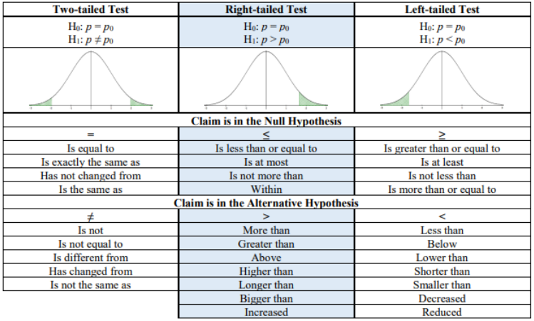
Figure \(\PageIndex{1}\): Types of Tests Based on Hypothesis and Keywords.
Note that the t-distribution is not used with proportions. We will use a standard normal z distribution for testing a proportion since this test uses the normal approximation to the binomial distribution (never use the t-distribution).
If you are doing a left-tailed z-test, the critical value will be negative. If you are performing a right-tailed z-test, the critical value will be positive. If you were performing a two-tailed z-test, then your critical values would be ±critical value. The p-value will always be a positive number between 0 and 1. The most important step in any method you use is setting up your null and alternative hypotheses. The critical values and p-value can be found using a standard normal distribution in the same way that we did for the one-sample z-test.
It has been found that 85.6% of all enrolled college and university students in the United States are undergraduates. A random sample of 500 enrolled college students in a particular state revealed that 420 of them were undergraduates. Is there sufficient evidence to conclude that the proportion differs from the national percentage? Use \(\alpha\) = 0.05. Show that all three methods of hypothesis testing yield the same results.
Solution
At this point, you should be more comfortable with the steps of a hypothesis test and not have to number each step, but know what each step means.
- State the Hypothesis and Identify the Claim: The keywords in this example, “proportion” and “differs,” lead to the following hypotheses and claim.
H0: p = 0.856
H1: p ≠ 0.856 (claim)
- Find the Critical Value: Look up the critical value in the table.
Use \(\alpha\) = 0.05 and look up the critical values in the table to get \( \pm 1.96\).
- Compute the Test Statistic: Before computing the test statistic, compute the sample proportion \(\hat{p}=\dfrac{420}{500}=0.84\) and q = 1 – 0.856 = 0.144.
\[z=\dfrac{\hat{p}-p}{\sqrt{\left(\dfrac{p \cdot q}{n}\right)}}=\dfrac{0.84-0.856}{\sqrt{\left(\dfrac{0.856 \cdot 0.144}{500}\right)}}=-1.02.\]
- Make the Decision: Draw and label the curve with the critical values and make the decision to reject or not reject the null hypothesis \((H_0)\).

State the decision. Since the test statistic is not in the shaded rejection area, do not reject H0.
- Summarize the Results: There is not enough evidence to conclude that the proportion of undergraduates in college for this state differs from the national average of 85.6%.
A California Community College claims that at least 30% of its students major in STEM fields. A student researcher believes that the proportion is greater than. To test this the researcher's, the researcher surveys a random sample of 120 students and finds that 45 of them are majoring in STEM.
At \( \alpha = 0.10 \), test the claim that the proportion of STEM majors at the college is greater than 30%.
Solution
- State the Hypothesis and Identify the Claim: The keywords in this example, “proportion” and “differs,” ead to the following hypotheses and claim.
H0: p = 0.3
H1: p > 0.3 (claim)
- Find the Critical Value: Look up the critical value in the table.
Use \(\alpha\) = 0.10 and look up the critical values in the table to get \( 1.28\).
- Compute the Test Statistic:
The sample proportions are \(\hat{p} = \dfrac{45}{120} = 0.375\) and q = 1 – p = 1 – 0.3 = 0.7
\[z=\dfrac{\hat{p}-p}{\sqrt{\left(\dfrac{p \cdot q}{n}\right)}}=\dfrac{0.375-0.3}{\sqrt{\left(\dfrac{0.3 \cdot 0.7}{120}\right)}}=1.79.\]
- Make the Decision: Draw and label the curve with the critical value and make the decision to reject or not reject the null hypothesis \((H_0)\).

Since the test statistic falls in the critical region, reject H0.
- Summarize the Results: There is enough evidence to support the researcher's claim that the proportion is greater than 30%.
It has been found that 85.6% of all enrolled college and university students in the United States are undergraduates. A random sample of 500 enrolled college students in a particular state revealed that 420 of them were undergraduates. Is there sufficient evidence to conclude that the proportion differs from the national percentage? Use \(\alpha\) = 0.05. Show that all three methods of hypothesis testing yield the same results.
Solution
- State the Hypothesis and Identify the Claim: The keywords in this example, “proportion” and “differs,” lead to the following hypotheses and claim.
H0: p = 0.856
H1: p ≠ 0.856 (claim)
- Compute the Test Statistic:
\(Z=\dfrac{\hat{p}-p}{\sqrt{\left(\dfrac{p \cdot q}{n}\right)}}=\dfrac{0.84-0.856}{\sqrt{\left(\dfrac{0.856 \cdot 0.144}{500}\right)}}=-1.019\)
- Compute the P-Value:
To find the p-value, we need to find the area to the left of z = –1.02 and the right of z = 1.02, and then add the areas together. First, find the area to the left of z = –1.02 using the Standard Normal Distribution Table is 0.1539. Then, double this area to get the p-value = 0.3078.
We can also find the p-value using the TI-84+ Graphing Calculator, although the final answer may be slightly different due to the rounding of the z-value. Use the steps below to compute the p-value. In this case, the p-value = 0.3082, which differs slightly from the value found in the table.
TI-84: Press the [STAT] key, arrow over to the [TESTS] menu, arrow down to the option [5:1-PropZTest] and press the [ENTER] key. Type in the hypothesized proportion (p), x, sample size, arrow over to the \(\neq\), <, > sign that is the same in the problem’s alternative hypothesis statement then press the [ENTER] key, arrow down to [Calculate] and press the [ENTER] key.

Figure \(\PageIndex{4}\): Output of Normal Area Function using TI-84+ Calculator.
- Make the Decision: Since the p-value > \(\alpha\), the decision is not to reject H0.
In this case, p-value = 0.3078 (table) or 0.3082 (calculator) > \( \alpha = 0.05 \) - reject H0.
- Summarize the Results: There is not enough evidence to conclude that the proportion of undergraduates in college for this state differs from the national average of 85.6%.
General Decision Rule for P-Value Method
- Reject H0 when the p-value ≤ \(\alpha\).
- Do not reject H0 when the p-value > \(\alpha\).
Authors
"8.5: z-Test for a Proportion" by Toros Berberyan, Tracy Nguyen, and Alfie Swan is licensed under CC BY-SA 4.0
Attributions
"8.4: Hypothesis Test for One Proportion" by Rachel Webb is licensed under CC BY-SA 4.0
Exercises
- According to a national health report, 11% of adults in the United States have diabetes. A health researcher believes the proportion is different in a particular city. To test this, the researcher surveys 200 randomly selected adults from the city and finds that 28 of them have diabetes. At \(\alpha = 0.10\), test the claim that the proportion of adults with diabetes in the city is different from the national rate of 11%. Using the traditional method.
Scan the QR code or click on it to open the MyOpenMath version of the above question with step-by-step guidance.
MyOpenMath is a free online learning platform designed to support math instruction through automated homework, quizzes, and assessments. You must register for MyOpenMath and sign in to view the question.

- According to a national health report, 11% of adults in the United States have diabetes. A health researcher believes the proportion is different in a particular city. To test this, the researcher surveys 200 randomly selected adults from the city and finds that 28 of them have diabetes. At \(\alpha = 0.10\), test the claim that the proportion of adults with diabetes in the city is different from the national rate of 11%. Using the p-value method.
Scan the QR code or click on it to open the MyOpenMath version of the above question with step-by-step guidance.
MyOpenMath is a free online learning platform designed to support math instruction through automated homework, quizzes, and assessments. You must register for MyOpenMath and sign in to view the question.

- In previous years, surveys showed that about 60% of adults reported going out for leisure activities on the weekends. Due to rising costs and economic concerns, a researcher believes this proportion has decreased. To test this claim, the researcher surveys 150 randomly selected adults and finds that 78 of them say they go out on weekends. At \(\alpha = 0.05 \), test the claim that the current proportion of people going out on weekends is less than 60%. Use the traditional method.
Scan the QR code or click on it to open the MyOpenMath version of the above question with step-by-step guidance.
MyOpenMath is a free online learning platform designed to support math instruction through automated homework, quizzes, and assessments. You must register for MyOpenMath and sign in to view the question.

- In previous years, surveys showed that about 60% of adults reported going out for leisure activities on the weekends. Due to rising costs and economic concerns, a researcher believes this proportion has decreased. To test this claim, the researcher surveys 150 randomly selected adults and finds that 78 of them say they go out on weekends. At \(\alpha = 0.05 \), test the claim that the current proportion of people going out on weekends is less than 60%. Use the p-value method.
Scan the QR code or click on it to open the MyOpenMath version of the above question with step-by-step guidance.
MyOpenMath is a free online learning platform designed to support math instruction through automated homework, quizzes, and assessments. You must register for MyOpenMath and sign in to view the question.

- A fitness influencer claims that more people are committing to daily workouts thanks to the rise of online fitness challenges and social media trends. Historically, only 25% of adults exercised daily. To test this claim, a sports magazine surveys 180 randomly selected adults and finds that 58 of them report exercising every single day. At the \(\alpha = 0.01\), test the influencer's claim that the proportion of people who exercise daily has increased. Use the traditional method.
Scan the QR code or click on it to open the MyOpenMath version of the above question with step-by-step guidance.
MyOpenMath is a free online learning platform designed to support math instruction through automated homework, quizzes, and assessments. You must register for MyOpenMath and sign in to view the question.

- A fitness influencer claims that more people are committing to daily workouts thanks to the rise of online fitness challenges and social media trends. Historically, only 25% of adults exercised daily. To test this claim, a sports magazine surveys 180 randomly selected adults and finds that 58 of them report exercising every single day. At the \(\alpha = 0.01\), test the influencer's claim that the proportion of people who exercise daily has increased. Use the p-value method.
Scan the QR code or click on it to open the MyOpenMath version of the above question with step-by-step guidance.
MyOpenMath is a free online learning platform designed to support math instruction through automated homework, quizzes, and assessments. You must register for MyOpenMath and sign in to view the question.

- Answers
-
If you are an instructor and want the solutions to all the exercise questions for each section, please email Toros Berberyan.