
11.5: Mean First Passage Time for Ergodic Chains
- Page ID
- 3176

\( \newcommand{\vecs}[1]{\overset { \scriptstyle \rightharpoonup} {\mathbf{#1}} } \)
\( \newcommand{\vecd}[1]{\overset{-\!-\!\rightharpoonup}{\vphantom{a}\smash {#1}}} \)
\( \newcommand{\id}{\mathrm{id}}\) \( \newcommand{\Span}{\mathrm{span}}\)
( \newcommand{\kernel}{\mathrm{null}\,}\) \( \newcommand{\range}{\mathrm{range}\,}\)
\( \newcommand{\RealPart}{\mathrm{Re}}\) \( \newcommand{\ImaginaryPart}{\mathrm{Im}}\)
\( \newcommand{\Argument}{\mathrm{Arg}}\) \( \newcommand{\norm}[1]{\| #1 \|}\)
\( \newcommand{\inner}[2]{\langle #1, #2 \rangle}\)
\( \newcommand{\Span}{\mathrm{span}}\)
\( \newcommand{\id}{\mathrm{id}}\)
\( \newcommand{\Span}{\mathrm{span}}\)
\( \newcommand{\kernel}{\mathrm{null}\,}\)
\( \newcommand{\range}{\mathrm{range}\,}\)
\( \newcommand{\RealPart}{\mathrm{Re}}\)
\( \newcommand{\ImaginaryPart}{\mathrm{Im}}\)
\( \newcommand{\Argument}{\mathrm{Arg}}\)
\( \newcommand{\norm}[1]{\| #1 \|}\)
\( \newcommand{\inner}[2]{\langle #1, #2 \rangle}\)
\( \newcommand{\Span}{\mathrm{span}}\) \( \newcommand{\AA}{\unicode[.8,0]{x212B}}\)
\( \newcommand{\vectorA}[1]{\vec{#1}} % arrow\)
\( \newcommand{\vectorAt}[1]{\vec{\text{#1}}} % arrow\)
\( \newcommand{\vectorB}[1]{\overset { \scriptstyle \rightharpoonup} {\mathbf{#1}} } \)
\( \newcommand{\vectorC}[1]{\textbf{#1}} \)
\( \newcommand{\vectorD}[1]{\overrightarrow{#1}} \)
\( \newcommand{\vectorDt}[1]{\overrightarrow{\text{#1}}} \)
\( \newcommand{\vectE}[1]{\overset{-\!-\!\rightharpoonup}{\vphantom{a}\smash{\mathbf {#1}}}} \)
\( \newcommand{\vecs}[1]{\overset { \scriptstyle \rightharpoonup} {\mathbf{#1}} } \)
\( \newcommand{\vecd}[1]{\overset{-\!-\!\rightharpoonup}{\vphantom{a}\smash {#1}}} \)
\(\newcommand{\avec}{\mathbf a}\) \(\newcommand{\bvec}{\mathbf b}\) \(\newcommand{\cvec}{\mathbf c}\) \(\newcommand{\dvec}{\mathbf d}\) \(\newcommand{\dtil}{\widetilde{\mathbf d}}\) \(\newcommand{\evec}{\mathbf e}\) \(\newcommand{\fvec}{\mathbf f}\) \(\newcommand{\nvec}{\mathbf n}\) \(\newcommand{\pvec}{\mathbf p}\) \(\newcommand{\qvec}{\mathbf q}\) \(\newcommand{\svec}{\mathbf s}\) \(\newcommand{\tvec}{\mathbf t}\) \(\newcommand{\uvec}{\mathbf u}\) \(\newcommand{\vvec}{\mathbf v}\) \(\newcommand{\wvec}{\mathbf w}\) \(\newcommand{\xvec}{\mathbf x}\) \(\newcommand{\yvec}{\mathbf y}\) \(\newcommand{\zvec}{\mathbf z}\) \(\newcommand{\rvec}{\mathbf r}\) \(\newcommand{\mvec}{\mathbf m}\) \(\newcommand{\zerovec}{\mathbf 0}\) \(\newcommand{\onevec}{\mathbf 1}\) \(\newcommand{\real}{\mathbb R}\) \(\newcommand{\twovec}[2]{\left[\begin{array}{r}#1 \\ #2 \end{array}\right]}\) \(\newcommand{\ctwovec}[2]{\left[\begin{array}{c}#1 \\ #2 \end{array}\right]}\) \(\newcommand{\threevec}[3]{\left[\begin{array}{r}#1 \\ #2 \\ #3 \end{array}\right]}\) \(\newcommand{\cthreevec}[3]{\left[\begin{array}{c}#1 \\ #2 \\ #3 \end{array}\right]}\) \(\newcommand{\fourvec}[4]{\left[\begin{array}{r}#1 \\ #2 \\ #3 \\ #4 \end{array}\right]}\) \(\newcommand{\cfourvec}[4]{\left[\begin{array}{c}#1 \\ #2 \\ #3 \\ #4 \end{array}\right]}\) \(\newcommand{\fivevec}[5]{\left[\begin{array}{r}#1 \\ #2 \\ #3 \\ #4 \\ #5 \\ \end{array}\right]}\) \(\newcommand{\cfivevec}[5]{\left[\begin{array}{c}#1 \\ #2 \\ #3 \\ #4 \\ #5 \\ \end{array}\right]}\) \(\newcommand{\mattwo}[4]{\left[\begin{array}{rr}#1 \amp #2 \\ #3 \amp #4 \\ \end{array}\right]}\) \(\newcommand{\laspan}[1]{\text{Span}\{#1\}}\) \(\newcommand{\bcal}{\cal B}\) \(\newcommand{\ccal}{\cal C}\) \(\newcommand{\scal}{\cal S}\) \(\newcommand{\wcal}{\cal W}\) \(\newcommand{\ecal}{\cal E}\) \(\newcommand{\coords}[2]{\left\{#1\right\}_{#2}}\) \(\newcommand{\gray}[1]{\color{gray}{#1}}\) \(\newcommand{\lgray}[1]{\color{lightgray}{#1}}\) \(\newcommand{\rank}{\operatorname{rank}}\) \(\newcommand{\row}{\text{Row}}\) \(\newcommand{\col}{\text{Col}}\) \(\renewcommand{\row}{\text{Row}}\) \(\newcommand{\nul}{\text{Nul}}\) \(\newcommand{\var}{\text{Var}}\) \(\newcommand{\corr}{\text{corr}}\) \(\newcommand{\len}[1]{\left|#1\right|}\) \(\newcommand{\bbar}{\overline{\bvec}}\) \(\newcommand{\bhat}{\widehat{\bvec}}\) \(\newcommand{\bperp}{\bvec^\perp}\) \(\newcommand{\xhat}{\widehat{\xvec}}\) \(\newcommand{\vhat}{\widehat{\vvec}}\) \(\newcommand{\uhat}{\widehat{\uvec}}\) \(\newcommand{\what}{\widehat{\wvec}}\) \(\newcommand{\Sighat}{\widehat{\Sigma}}\) \(\newcommand{\lt}{<}\) \(\newcommand{\gt}{>}\) \(\newcommand{\amp}{&}\) \(\definecolor{fillinmathshade}{gray}{0.9}\)In this section we consider two closely related descriptive quantities of interest for ergodic chains: the mean time to return to a state and the mean time to go from one state to another state.
Let \(\mathbf{P}\) be the transition matrix of an ergodic chain with states \(s_1\), \(s_2\), …, \(s_r\). Let \(\mathbf {w} = (w_1,w_2,\ldots,w_r)\) be the unique probability vector such that \(\mathbf {w} \mathbf {P} = \mathbf {w}\). Then, by the Law of Large Numbers for Markov chains, in the long run the process will spend a fraction \(w_j\) of the time in state \(s_j\). Thus, if we start in any state, the chain will eventually reach state \(s_j\); in fact, it will be in state \(s_j\) infinitely often.
Another way to see this is the following: Form a new Markov chain by making \(s_j\) an absorbing state, that is, define \(p_{jj} = 1\). If we start at any state other than \(s_j\), this new process will behave exactly like the original chain up to the first time that state \(s_j\) is reached. Since the original chain was an ergodic chain, it was possible to reach \(s_j\) from any other state. Thus the new chain is an absorbing chain with a single absorbing state \(s_j\) that will eventually be reached. So if we start the original chain at a state \(s_i\) with \(i \ne j\), we will eventually reach the state \(s_j\).
Let \(\mathbf{N}\) be the fundamental matrix for the new chain. The entries of \(\mathbf{N}\) give the expected number of times in each state before absorption. In terms of the original chain, these quantities give the expected number of times in each of the states before reaching state \(s_j\) for the first time. The \(i\)th component of the vector \(\mathbf {N} \mathbf {c}\) gives the expected number of steps before absorption in the new chain, starting in state \(s_i\). In terms of the old chain, this is the expected number of steps required to reach state \(s_j\) for the first time starting at state \(s_i\).
Mean First Passage Time
If an ergodic Markov chain is started in state \(s_i\), the expected number of steps to reach state \(s_j\) for the first time is called the from \(s_i\) to \(s_j\). It is denoted by \(m_{ij}\). By convention \(m_{ii} = 0\).
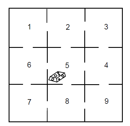
Let us return to the maze example (Example 11.3.3). We shall make this ergodic chain into an absorbing chain by making state 5 an absorbing state. For example, we might assume that food is placed in the center of the maze and once the rat finds the food, he stays to enjoy it (see Figure [\(\PageIndex{1}\)).
The new transition matrix in canonical form is
\[\mathbf{P}= \begin{matrix} & \begin{matrix}1&&2&&3&&4&&5&&6&&7&&8&&9\end{matrix} \\\begin{matrix}1\\2\\3\\4\\5\\6\\7\\8\\9\end{matrix} &
\left(\begin{array}{cccccccc|c}
0 & 1 / 2 & 0 & 0 & 1 / 2 & 0 & 0 & 0 & 0 \\
1 / 3 & 0 & 1 / 3 & 0 & 0 & 0 & 0 & 0 & 1 / 3 \\
0 & 1 / 2 & 0 & 1 / 2 & 0 & 0 & 0 & 0 & 0 \\
0 & 0 & 1 / 3 & 0 & 0 & 1 / 3 & 0 & 1 / 3 & 1 / 3 \\
1 / 3 & 0 & 0 & 0 & 0 & 0 & 0 & 0 & 1 / 3 \\
0 & 0 & 0 & 0 & 1 / 2 & 0 & 1 / 2 & 0 & 0 \\
0 & 0 & 0 & 0 & 0 & 1 / 3 & 0 & 1 / 3 & 1 / 3 \\
0 & 0 & 0 & 1 / 2 & 0 & 0 & 1 / 2 & 0 & 0 \\
\hline 0 & 0 & 0 & 0 & 0 & 0 & 0 & 0 & 1
\end{array}\right)\end{matrix}\]
If we compute the fundamental matrix \(\mathbf{N}\), we obtain
\[\mathbf {N} = \frac18 \pmatrix{ 14 & 9 & 4 & 3 & 9 & 4 & 3 & 2 \cr 6 & 14 & 6 & 4 & 4 & 2 & 2 & 2 \cr 4 & 9 & 14 & 9 & 3 & 2 & 3 & 4 \cr 2 & 4 & 6 & 14 & 2 & 2 & 4 & 6 \cr 6 & 4 & 2 & 2 & 14 & 6 & 4 & 2 \cr 4 & 3 & 2 & 3 & 9 & 14 & 9 & 4 \cr 2 & 2 & 2 & 4 & 4 & 6 & 14 & 6 \cr 2 & 3 & 4 & 9 & 3 & 4 & 9 & 14 \cr}\ .\]
The expected time to absorption for different starting states is given by the vector \(\mathbf {N} \mathbf {c}\), where
\[\mathbf {N} \mathbf {c} = \pmatrix{ 6 \cr 5 \cr 6 \cr 5 \cr 5 \cr 6 \cr 5 \cr 6 \cr}\ .\]
We see that, starting from compartment 1, it will take on the average six steps to reach food. It is clear from symmetry that we should get the same answer for starting at state 3, 7, or 9. It is also clear that it should take one more step, starting at one of these states, than it would starting at 2, 4, 6, or 8. Some of the results obtained from \(\mathbf{N}\) are not so obvious. For instance, we note that the expected number of times in the starting state is 14/8 regardless of the state in which we start.
Mean Recurrence Time
A quantity that is closely related to the mean first passage time is the mean recurrence time defined as follows. Assume that we start in state \(s_i\); consider the length of time before we return to \(s_i\) for the first time. It is clear that we must return, since we either stay at \(s_i\) the first step or go to some other state \(s_j\), and from any other state \(s_j\), we will eventually reach \(s_i\) because the chain is ergodic.
If an ergodic Markov chain is started in state \(s_i\), the expected number of steps to return to \(s_i\) for the first time is the mean recurrance time for \(s_i\). It is denoted by \(r_i\).
We need to develop some basic properties of the mean first passage time. Consider the mean first passage time from \(s_i\) to \(s_j\); assume that \(i \ne j\). This may be computed as follows: take the expected number of steps required given the outcome of the first step, multiply by the probability that this outcome occurs, and add. If the first step is to \(s_j\), the expected number of steps required is 1; if it is to some other state \(s_k\), the expected number of steps required is \(m_{kj}\) plus 1 for the step already taken. Thus,
\[m_{ij} = p_{ij} + \sum_{k \ne j} p_{ik}(m_{kj} + 1)\ ,\]
or, since \(\sum_k p_{ik} = 1\),
\[m_{ij} = 1 + \sum_{k \ne j}p_{ik} m_{kj}\ .\label{eq 11.5.1}\]
Similarly, starting in \(s_i\), it must take at least one step to return. Considering all possible first steps gives us
\[\begin{aligned} r_i &=& \sum_k p_{ik}(m_{ki} + 1) \\ &=& 1 + \sum_k p_{ik} m_{ki}\ .\label{eq 11.5.2}\end{aligned}\]
Mean First Passage Matrix and Mean Recurrence Matrix
Let us now define two matrices \(\mathbf{M}\) and \(\mathbf{D}\). The \(ij\)th entry \(m_{ij}\) of \(\mathbf{M}\) is the mean first passage time to go from \(s_i\) to \(s_j\) if \(i \ne j\); the diagonal entries are 0. The matrix \(\mathbf{M}\) is called the mean first passage matrix. The matrix \(\mathbf{D}\) is the matrix with all entries 0 except the diagonal entries \(d_{ii} = r_i\). The matrix \(\mathbf{D}\) is called the mean recurrence matrix. Let \(\mathbf {C}\) be an \(r \times r\) matrix with all entries 1. Using Equation [eq 11.5.1] for the case \(i \ne j\) and Equation [eq 11.5.2] for the case \(i = j\), we obtain the matrix equation \[\mathbf{M} = \mathbf{P} \mathbf{M} + \mathbf{C} - \mathbf{D}\ , \label{eq 11.5.3}\] or \[(\mathbf{I} - \mathbf{P}) \mathbf{M} = \mathbf{C} - \mathbf{D}\ . \label{eq 11.5.4}\] Equation [eq 11.5.4] with \(m_{ii} = 0\) implies Equations [eq 11.5.1] and [eq 11.5.2]. We are now in a position to prove our first basic theorem.
For an ergodic Markov chain, the mean recurrence time for state \(s_i\) is \(r_i = 1/w_i\), where \(w_i\) is the \(i\)th component of the fixed probability vector for the transition matrix.
Proof. Multiplying both sides of Equation \(\PageIndex{6}\) by \(\mathbf{w}\) and using the fact that
\[\mathbf {w}(\mathbf {I} - \mathbf {P}) = \mathbf {0}\]
gives
\[\mathbf {w} \mathbf {C} - \mathbf {w} \mathbf {D} = \mathbf {0}\ .\]
Here \(\mathbf {w} \mathbf {C}\) is a row vector with all entries 1 and \(\mathbf {w} \mathbf {D}\) is a row vector with \(i\)th entry \(w_i r_i\). Thus
\[(1,1,\ldots,1) = (w_1r_1,w_2r_2,\ldots,w_nr_n)\] and \[r_i = 1/w_i\ ,\]
as was to be proved.
For an ergodic Markov chain, the components of the fixed probability vector w are strictly positive. We know that the values of \(r_i\) are finite and so \(w_i = 1/r_i\) cannot be 0.
In Section 11.3 we found the fixed probability vector for the maze example to be
\[\mathbf {w} = \pmatrix{ \frac1{12} & \frac18 & \frac1{12} & \frac18 & \frac16 & \frac18 & \frac1{12} & \frac18 & \frac1{12}}\ .\]
Hence, the mean recurrence times are given by the reciprocals of these probabilities. That is,
\[\mathbf {r} = \pmatrix{ 12 & 8 & 12 & 8 & 6 & 8 & 12 & 8 & 12 }\ .\]
Returning to the Land of Oz, we found that the weather in the Land of Oz could be represented by a Markov chain with states rain, nice, and snow. In Section 1.3 we found that the limiting vector was \(\mathbf {w} = (2/5,1/5,2/5)\). From this we see that the mean number of days between rainy days is 5/2, between nice days is 5, and between snowy days is 5/2.
Fundamental Matrix
We shall now develop a fundamental matrix for ergodic chains that will play a role similar to that of the fundamental matrix \(\mathbf {N} = (\mathbf {I} - \mathbf {Q})^{-1}\) for absorbing chains. As was the case with absorbing chains, the fundamental matrix can be used to find a number of interesting quantities involving ergodic chains. Using this matrix, we will give a method for calculating the mean first passage times for ergodic chains that is easier to use than the method given above. In addition, we will state (but not prove) the Central Limit Theorem for Markov Chains, the statement of which uses the fundamental matrix.
We begin by considering the case that is the transition matrix of a regular Markov chain. Since there are no absorbing states, we might be tempted to try \(\mathbf {Z} = (\mathbf {I} - \mathbf {P})^{-1}\) for a fundamental matrix. But \(\mathbf {I} - \mathbf {P}\) does not have an inverse. To see this, recall that a matrix \(\mathbf{R}\) has an inverse if and only if \(\mathbf {R} \mathbf {x} = \mathbf {0}\) implies \(\mathbf {x} = \mathbf {0}\). But since \(\mathbf {P} \mathbf {c} = \mathbf {c}\) we have \((\mathbf {I} - \mathbf {P})\mathbf {c} = \mathbf {0}\), and so \(\mathbf {I} - \mathbf {P}\) does not have an inverse.
We recall that if we have an absorbing Markov chain, and is the restriction of the transition matrix to the set of transient states, then the fundamental matrix could be written as
\[\mathbf {N} = \mathbf {I} + \mathbf {Q} + \mathbf {Q}^2 + \cdots\ .\]
The reason that this power series converges is that \(\mathbf {Q}^n \rightarrow 0\), so this series acts like a convergent geometric series.
This idea might prompt one to try to find a similar series for regular chains. Since we know that \(\mathbf {P}^n \rightarrow \mathbf {W}\), we might consider the series
\[\mathbf {I} + (\mathbf {P} -\mathbf {W}) + (\mathbf {P}^2 - \mathbf{W}) + \cdots\ .\label{eq 11.5.8}\]
We now use special properties of and to rewrite this series. The special properties are: 1) \(\mathbf {P}\mathbf {W} = \mathbf {W}\), and 2) \(\mathbf {W}^k = \mathbf {W}\) for all positive integers \(k\). These facts are easy to verify, and are left as an exercise (see Exercise [exer 11.5.28]). Using these facts, we see that
\[\begin{aligned} (\mathbf {P} - \mathbf {W})^n &=& \sum_{i = 0}^n (-1)^i{n \choose i}\mathbf {P}^{n-i}\mathbf {W}^i \\ &=& \mathbf {P}^n + \sum_{i = 1}^n (-1)^i{n \choose i} \mathbf {W}^i \\ &=& \mathbf {P}^n + \sum_{i = 1}^n (-1)^i{n \choose i} \mathbf {W} \\ &=& \mathbf {P}^n + \Biggl(\sum_{i = 1}^n (-1)^i{n \choose i}\Biggr) \mathbf {W}\ .\end{aligned}\]
If we expand the expression \((1-1)^n\), using the Binomial Theorem, we obtain the expression in parenthesis above, except that we have an extra term (which equals 1). Since \((1-1)^n = 0\), we see that the above expression equals -1. So we have
\[(\mathbf {P} - \mathbf {W})^n = \mathbf {P}^n - \mathbf {W}\ ,\] for all \(n \ge 1\).
We can now rewrite the series in Eq. \(\PageIndex{7}\) as \[\mathbf {I} + (\mathbf {P} - \mathbf {W}) + (\mathbf {P} - \mathbf {W})^2 + \cdots\ .\] Since the \(n\)th term in this series is equal to \(\mathbf {P}^n - \mathbf {W}\), the \(n\)th term goes to 0 as \(n\) goes to infinity. This is sufficient to show that this series converges, and sums to the inverse of the matrix \(\mathbf {I} - \mathbf {P} + \mathbf {W}\). We call this inverse the associated with the chain, and we denote it by .
In the case that the chain is ergodic, but not regular, it is not true that \(\mathbf {P}^n \rightarrow \mathbf {W}\) as \(n \rightarrow \infty\). Nevertheless, the matrix \(\mathbf {I} - \mathbf {P} + \mathbf {W}\) still has an inverse, as we will now show.
TLet be the transition matrix of an ergodic chain, and let be the matrix all of whose rows are the fixed probability row vector for . Then the matrix
\[\mathbf {I} - \mathbf {P} + \mathbf {W}\]
has an inverse.
Proof. Let \(\mathbf{x}\) be a column vector such that
\[(\mathbf {I} - \mathbf {P} + \mathbf {W})\mathbf {x} = \mathbf {0}\ .\]
To prove the proposition, it is sufficient to show that must be the zero vector. Multiplying this equation by \(\mathbf{w}\) and using the fact that \(\mathbf{w}(\mathbf{I} - \mathbf{ P}) = \mathbf{0}\) and \(\mathbf{w} \mathbf{W} = \mathbf {w}\), we have
\[\mathbf {w}(\mathbf {I} - \mathbf {P} + \mathbf {W})\mathbf {x} = \mathbf {w} \mathbf {x} = \mathbf {0}\ .\]
Therefore,
\[(\mathbf {I} - \mathbf {P})\mathbf {x} = \mathbf {0}\ .\]
But this means that \(\mathbf {x} = \mathbf {P} \mathbf {x}\) is a fixed column vector for \(\mathbf{P}\). By Theorem 11.3.4, this can only happen if \(\mathbf{x}\) is a constant vector. Since \(\mathbf {w}\mathbf {x} = 0\), and has strictly positive entries, we see that \(\mathbf {x} = \mathbf {0}\). This completes the proof.
As in the regular case, we will call the inverse of the matrix \(\mathbf {I} - \mathbf {P} + \mathbf {W}\) the for the ergodic chain with transition matrix , and we will use to denote this fundamental matrix.
Let \(\mathbf{P}\) be the transition matrix for the weather in the Land of Oz. Then
\[\begin{aligned} \mathbf{I} - \mathbf{P} + \mathbf{W} &=& \pmatrix{ 1 & 0 & 0\cr 0 & 1 & 0\cr 0 & 0 & 1\cr} - \pmatrix{ 1/2 & 1/4 & 1/4\cr 1/2 & 0 & 1/2\cr 1/4 & 1/4 & 1/2\cr} + \pmatrix{ 2/5 & 1/5 & 2/5\cr 2/5 & 1/5 & 2/5\cr 2/5 & 1/5 & 2/5\cr} \cr &=& \pmatrix{ 9/10 & -1/20 & 3/20\cr -1/10 & 6/5 & -1/10\cr 3/20 & -1/20 & 9/10\cr}\ ,\cr\end{aligned}\]
so
\[\mathbf{Z} = (\mathbf{I} - \mathbf{P} + \mathbf{W})^{-1} = \pmatrix{ 86/75 & 1/25 & -14/75\cr 2/25 & 21/25 & 2/25\cr -14/75 & 1/25 & 86/75\cr}\ .\]
Using the Fundamental Matrix to Calculate the Mean First Passage Matrix
We shall show how one can obtain the mean first passage matrix from the fundamental matrix for an ergodic Markov chain. Before stating the theorem which gives the first passage times, we need a few facts about .
Let \(\mathbf{Z} = (\mathbf{I} - \mathbf{P} + \mathbf{W})^{-1}\), and let \(\mathbf{c}\) be a column vector of all 1’s. Then
\[\mathbf{Z}\mathbf{c} = \mathbf{c}\ ,\] \[\mathbf{w}\mathbf{Z} = \mathbf{w}\ ,\]
and
\[\mathbf{Z}(\mathbf{I} - \mathbf{P}) = \mathbf{I} - \mathbf{W}\ .\]
Proof. Since \(\mathbf{P}\mathbf{c} = \mathbf{c}\) and \(\mathbf{W}\mathbf{c} = \mathbf{c}\),
\[\mathbf{c} = (\mathbf{I} - \mathbf{P} + \mathbf{W}) \mathbf{c}\ .\]
If we multiply both sides of this equation on the left by \(\mathbf{Z}\), we obtain
\[\mathbf{Z}\mathbf{c} = \mathbf{c}\ .\]
Similarly, since \(\mathbf{w}\mathbf{P} = \mathbf{w}\) and \(\mathbf{w}\mathbf{W} = \mathbf{w}\),
\[\mathbf{w} = \mathbf{w}(\mathbf{I} - \mathbf{P} + \mathbf{W})\ .\]
If we multiply both sides of this equation on the right by \(\mathbf{Z}\), we obtain
\[\mathbf{w}\mathbf{Z} = \mathbf{w}\ .\]
Finally, we have
\[\begin{aligned} (\mathbf{I} - \mathbf{P} + \mathbf{W})(\mathbf{I} - \mathbf{W}) &=& \mathbf{I} - \mathbf{W} - \mathbf{P} + \mathbf{W} + \mathbf{W} - \mathbf{W}\\ &=& \mathbf{I} - \mathbf{P}\ .\end{aligned}\]
Multiplying on the left by , we obtain \[\mathbf{I} - \mathbf{W} = \mathbf{Z}(\mathbf{I} - \mathbf{P})\ .\]
This completes the proof.
The following theorem shows how one can obtain the mean first passage times from the fundamental matrix.
The mean first passage matrix \(\mathbf{M}\) for an ergodic chain is determined from the fundamental matrix \(\mathbf{Z}\) and the fixed row probability vector \(\mathbf{w}\) by
\[m_{ij} = \frac{z_{jj} - z_{ij}}{w_j}\ .\]
Proof. We showed in Equation \(\PageIndex{6}\) that
\[(\mathbf {I} - \mathbf {P})\mathbf {M} = \mathbf {C} - \mathbf {D}\ .\]
Thus,
\[\mathbf {Z}(\mathbf {I} - \mathbf {P})\mathbf {M} = \mathbf {Z} \mathbf {C} - \mathbf {Z} \mathbf {D}\ ,\]
and from Lemma \(\PageIndex{1}\),
\[\mathbf {Z}(\mathbf {I} - \mathbf {P})\mathbf {M} = \mathbf {C} - \mathbf {Z} \mathbf {D}\ .\]
Again using Lemma \(\PageIndex{1}\), we have
\[\mathbf {M} - \mathbf{W}\mathbf {M} = \mathbf {C} - \mathbf {Z} \mathbf {D}\]
or
\[\mathbf {M} = \mathbf {C} - \mathbf {Z} \mathbf {D} + \mathbf{W}\mathbf {M}\ .\]
From this equation, we see that
\[m_{ij} = 1 - z_{ij}r_j + (\mathbf{w} \mathbf{M})_j\ . \label{eq 11.5.6}\]
But \(m_{jj} = 0\), and so
\[0 = 1 - z_{jj}r_j + (\mathbf {w} \mathbf {M})_j\ ,\]
or
\[(\mathbf{w} \mathbf{M})_j = z_{jj}r_j - 1\ . \label{eq 11.5.7}\]
From Equations \(\PageIndex{8}\) and \(\PageIndex{9}\), we have
\[m_{ij} = (z_{jj} - z_{ij}) \cdot r_j\ .\]
Since \(r_j = 1/w_j\),
\[m_{ij} = \frac{z_{jj} - z_{ij}}{w_j}\ .\]
(Example \(\PageIndex{3}\)continued) In the Land of Oz example, we find that
\[\mathbf{Z} = (\mathbf{I} - \mathbf{P} + \mathbf{W})^{-1} = \pmatrix{ 86/75 & 1/25 & -14/75\cr 2/25 & 21/25 & 2/25\cr -14/75 & 1/25 & 86/75\cr}\ .\]
We have also seen that \(\mathbf {w} = (2/5,1/5, 2/5)\). So, for example,
\[\begin{aligned} m_{12} &=& \frac{z_{22} - z_{12}}{w_2} \\ &=& \frac{21/25 - 1/25}{1/5} \\ &=& 4\ ,\\\end{aligned}\]
by Theorem \(\PageIndex{2}\). Carrying out the calculations for the other entries of \(\mathbf{M}\), we obtain
\[\mathbf {M} = \pmatrix{ 0 & 4 & 10/3\cr 8/3 & 0 & 8/3\cr 10/3 & 4 & 0\cr}\ .\]
Computation
The program ErgodicChain calculates the fundamental matrix, the fixed vector, the mean recurrence matrix \(\mathbf{D}\), and the mean first passage matrix \(\mathbf{M}\). We have run the program for the Ehrenfest urn model (Example [exam 11.1.6]). We obtain:
\[\mathbf{P}= \begin{matrix} & \begin{matrix}0&&&1&&&2&&&3&&&4\end{matrix} \\\begin{matrix}0\\1\\2\\3\\4 \end{matrix} &
\left(\begin{array}{ccccc}
.0000 & 1.0000 & .0000 & .0000 & .0000 \\
.2500 & .0000 & .7500 & .0000 & .0000 \\
.0000 & .5000 & .0000 & .5000 & .0000 \\
.0000 & .0000 & .7500 & .0000 & .2500 \\
.0000 & .0000 & .0000 & 1.0000 & .0000
\end{array}\right)\end{matrix}\]
\[\mathbf{w}= \begin{matrix} & \begin{matrix}0&&&1&&&2&&&3&&&4\end{matrix} \\ & \begin{pmatrix}
.0625 & .2500 & .3750 & .2500 & .0625 \\
\end{pmatrix}\\\end{matrix}\]
\[\mathbf{r}= \begin{matrix} & \begin{matrix}0&&&&1&&&&2&&&3&&&4\end{matrix} \\ & \begin{pmatrix}
16.0000 & 4.0000 & 2.6667 & 4.0000 & 16.0000 \\
\end{pmatrix}\\\end{matrix}\]
\[\mathbf{M}= \begin{matrix} & \begin{matrix}0&&&1&&&2&&&3&&&4\end{matrix} \\\begin{matrix}0\\1\\2\\3\\4 \end{matrix} &
\left(\begin{array}{ccccc}
.00000 & 1.0000 & 2.6667 & 6.3333 & 21.3333 \\
15.0000 & .0000 & 1.6667 & 5.3333 & 20.3333 \\
18.6667 & 3.6667 & .0000 & 3.6667 & 18.6667 \\
20.3333 & 5.3333 & 1.6667 & .0000 & 15.0000 \\
21.3333 & 6.3333 & 2.6667 & 1.0000 & .0000
\end{array}\right)\end{matrix}\]
From the mean first passage matrix, we see that the mean time to go from 0 balls in urn 1 to 2 balls in urn 1 is 2.6667 steps while the mean time to go from 2 balls in urn 1 to 0 balls in urn 1 is 18.6667. This reflects the fact that the model exhibits a central tendency. Of course, the physicist is interested in the case of a large number of molecules, or balls, and so we should consider this example for \(n\) so large that we cannot compute it even with a computer.
Ehrenfest Model
(Example \(\PageIndex{5}\)] continued) Let us consider the Ehrenfest model (see Example 11.1.6) for gas diffusion for the general case of \(2n\) balls. Every second, one of the \(2n\) balls is chosen at random and moved from the urn it was in to the other urn. If there are \(i\) balls in the first urn, then with probability \(i/2n\) we take one of them out and put it in the second urn, and with probability \((2n - i)/2n\) we take a ball from the second urn and put it in the first urn. At each second we let the number \(i\) of balls in the first urn be the state of the system. Then from state \(i\) we can pass only to state \(i - 1\) and \(i + 1\), and the transition probabilities are given by
\[p_{i j}=\left\{\begin{array}{cc}
\frac{i}{2 n}, & \text { if } j=i-1 \\
1-\frac{i}{2 n}, & \text { if } j=i+1 \\
0, & \text { otherwise. }
\end{array}\right.\]
This defines the transition matrix of an ergodic, non-regular Markov chain (see Exercise \(\PageIndex{15}\)). Here the physicist is interested in long-term predictions about the state occupied. In Example 11.3.4, we gave an intuitive reason for expecting that the fixed vector \(\mathbf{w}\) is the binomial distribution with parameters \(2n\) and \(1/2\). It is easy to check that this is correct. So,
\[w_i=\dfrac{\left(\begin{array}{c} 2 n \\ i \end{array}\right)}{2^{2 n}}\]
Thus the mean recurrence time for state \(i\) is
\[ r_i=\frac{2^{2 n}}{\left(\begin{array}{c} 2 n \\ i \end{array}\right)} \]
Consider in particular the central term \(i = n\). We have seen that this term is approximately \(1/\sqrt{\pi n}\). Thus we may approximate \(r_n\) by \(\sqrt{\pi n}\).
This model was used to explain the concept of reversibility in physical systems. Assume that we let our system run until it is in equilibrium. At this point, a movie is made, showing the system’s progress. The movie is then shown to you, and you are asked to tell if the movie was shown in the forward or the reverse direction. It would seem that there should always be a tendency to move toward an equal proportion of balls so that the correct order of time should be the one with the most transitions from \(i\) to \(i - 1\) if \(i > n\) and \(i\) to \(i + 1\) if \(i < n\).

In Figure \(\PageIndex{2}\) we show the results of simulating the Ehrenfest urn model for the case of \(n = 50\) and 1000 time units, using the program EhrenfestUrn. The top graph shows these results graphed in the order in which they occurred and the bottom graph shows the same results but with time reversed. There is no apparent difference.
We note that if we had not started in equilibrium, the two graphs would typically look quite different.
Reversibility
If the Ehrenfest model is started in equilibrium, then the process has no apparent time direction. The reason for this is that this process has a property called Define \(X_n\) to be the number of balls in the left urn at step \(n\). We can calculate, for a general ergodic chain, the reverse transition probability:
\[\begin{aligned} P(X_{n - 1} = j | X_n = i) &=& \frac{P(X_{n - 1} = j,X_n = i)}{P(X_n = i)} \\ &=& \frac{P(X_{n - 1} = j) P(X_n = i | X_{n - 1} = j)}{P(X_n = i)} \\ &=& \frac{P(X_{n - 1} = j) p_{ji}}{P(X_n = i)}\ .\\\end{aligned}\]
In general, this will depend upon \(n\), since \(P(X_n = j)\) and also \(P(X_{n - 1} = j)\) change with \(n\). However, if we start with the vector \(\mathbf{w}\) or wait until equilibrium is reached, this will not be the case. Then we can define \[p_{ij}^* = \frac{w_j p_{ji}}{w_i}\] as a transition matrix for the process watched with time reversed.
Let us calculate a typical transition probability for the reverse chain \(\mathbf{ P}^* = \{p_{ij}^*\}\) in the Ehrenfest model. For example,
\begin{aligned}
p_{i, i-1}^* & =\frac{w_{i-1} p_{i-1, i}}{w_i}=\frac{\left(\begin{array}{c}
2 n \\
i-1
\end{array}\right)}{2^{2 n}} \times \frac{2 n-i+1}{2 n} \times \frac{2^{2 n}}{\left(\begin{array}{c}
2 n \\
i
\end{array}\right)} \\
& =\frac{(2 n) !}{(i-1) !(2 n-i+1) !} \times \frac{(2 n-i+1) i !(2 n-i) !}{2 n(2 n) !} \\
& =\frac{i}{2 n}=p_{i, i-1} .
\end{aligned}
Similar calculations for the other transition probabilities show that \(\mathbf {P}^* = \mathbf {P}\). When this occurs the process is called Clearly, an ergodic chain is reversible if, and only if, for every pair of states \(s_i\) and \(s_j\), \(w_i p_{ij} = w_j p_{ji}\). In particular, for the Ehrenfest model this means that \(w_i p_{i,i - 1} = w_{i - 1} p_{i - 1,i}\). Thus, in equilibrium, the pairs \((i, i - 1)\) and \((i - 1, i)\) should occur with the same frequency. While many of the Markov chains that occur in applications are reversible, this is a very strong condition. In Exercise [exer 11.5.12] you are asked to find an example of a Markov chain which is not reversible.
The Central Limit Theorem for Markov Chains
Suppose that we have an ergodic Markov chain with states \(s_1, s_2, \ldots, s_k\). It is natural to consider the distribution of the random variables \(S^{(n)}_j\), which denotes the number of times that the chain is in state \(s_j\) in the first \(n\) steps. The \(j\)th component \(w_j\) of the fixed probability row vector \(\mathbf{w}\) is the proportion of times that the chain is in state \(s_j\) in the long run. Hence, it is reasonable to conjecture that the expected value of the random variable \(S^{(n)}_j\), as \(n \rightarrow \infty\), is asymptotic to \(nw_j\), and it is easy to show that this is the case (see Exercise [exer 11.5.29]).
It is also natural to ask whether there is a limiting distribution of the random variables \(S^{(n)}_j\). The answer is yes, and in fact, this limiting distribution is the normal distribution. As in the case of independent trials, one must normalize these random variables. Thus, we must subtract from \(S^{(n)}_j\) its expected value, and then divide by its standard deviation. In both cases, we will use the asymptotic values of these quantities, rather than the values themselves. Thus, in the first case, we will use the value \(nw_j\). It is not so clear what we should use in the second case. It turns out that the quantity \[\sigma_j^2 = 2w_jz_{jj} - w_j - w_j^2 \label{eq 11.5.9}\] represents the asymptotic variance. Armed with these ideas, we can state the following theorem.
For an ergodic chain, for any real numbers \(r < s\), we have
\[ P\left(r<\frac{S_j^{(n)}-n w_j}{\sqrt{n \sigma_j^2}}<s\right) \rightarrow \frac{1}{\sqrt{2 \pi}} \int_r^s e^{-x^2 / 2} d x \]
as \(n \rightarrow \infty\), for any choice of starting state, where \(\sigma_j^2\) is the quantity defined in Equation 11.1.10.
Historical Remarks
Markov chains were introduced by Andreĭ Andreevich Markov (1856–1922) and were named in his honor. He was a talented undergraduate who received a gold medal for his undergraduate thesis at St. Petersburg University. Besides being an active research mathematician and teacher, he was also active in politics and patricipated in the liberal movement in Russia at the beginning of the twentieth century. In 1913, when the government celebrated the 300th anniversary of the House of Romanov family, Markov organized a counter-celebration of the 200th anniversary of Bernoulli’s discovery of the Law of Large Numbers.
Markov was led to develop Markov chains as a natural extension of sequences of independent random variables. In his first paper, in 1906, he proved that for a Markov chain with positive transition probabilities and numerical states the average of the outcomes converges to the expected value of the limiting distribution (the fixed vector). In a later paper he proved the central limit theorem for such chains. Writing about Markov, A. P. Youschkevitch remarks:
Markov arrived at his chains starting from the internal needs of probability theory, and he never wrote about their applications to physical science. For him the only real examples of the chains were literary texts, where the two states denoted the vowels and consonants.19
In a paper written in 1913,20 Markov chose a sequence of 20,000 letters from Pushkin’s to see if this sequence can be approximately considered a simple chain. He obtained the Markov chain with transition matrix
\[\mathbf{P}^6= \begin{matrix} & \begin{matrix}vowel&consonant\end{matrix} \\\begin{matrix}vowel\\consonant \end{matrix} & \begin{pmatrix}
.128&&& .872 \\
.663 &&&.337
\end{pmatrix}\\\end{matrix}\]
The fixed vector for this chain is \((.432, .568)\), indicating that we should expect about 43.2 percent vowels and 56.8 percent consonants in the novel, which was borne out by the actual count.
Claude Shannon considered an interesting extension of this idea in his book 21 in which he developed the information-theoretic concept of entropy. Shannon considers a series of Markov chain approximations to English prose. He does this first by chains in which the states are letters and then by chains in which the states are words. For example, for the case of words he presents first a simulation where the words are chosen independently but with appropriate frequencies.
REPRESENTING AND SPEEDILY IS AN GOOD APT OR COME CAN DIFFERENT NATURAL HERE HE THE A IN CAME THE TO OF TO EXPERT GRAY COME TO FURNISHES THE LINE MESSAGE HAD BE THESE.
He then notes the increased resemblence to ordinary English text when the words are chosen as a Markov chain, in which case he obtains
THE HEAD AND IN FRONTAL ATTACK ON AN ENGLISH WRITER THAT THE CHARACTER OF THIS POINT IS THEREFORE ANOTHER METHOD FOR THE LETTERS THAT THE TIME OF WHO EVER TOLD THE PROBLEM FOR AN UNEXPECTED.
A simulation like the last one is carried out by opening a book and choosing the first word, say it is Then the book is read until the word appears again and the word after this is chosen as the second word, which turned out to be The book is then read until the word appears again and the next word, is chosen, and so on.
Other early examples of the use of Markov chains occurred in Galton’s study of the problem of survival of family names in 1889 and in the Markov chain introduced by P. and T. Ehrenfest in 1907 for diffusion. Poincaré in 1912 dicussed card shuffling in terms of an ergodic Markov chain defined on a permutation group. Brownian motion, a continuous time version of random walk, was introducted in 1900–1901 by L. Bachelier in his study of the stock market, and in 1905–1907 in the works of A. Einstein and M. Smoluchowsky in their study of physical processes.
One of the first systematic studies of finite Markov chains was carried out by M. Frechet.22 The treatment of Markov chains in terms of the two fundamental matrices that we have used was developed by Kemeny and Snell 23 to avoid the use of eigenvalues that one of these authors found too complex. The fundamental matrix \(\mathbf{N}\) occurred also in the work of J. L. Doob and others in studying the connection between Markov processes and classical potential theory. The fundamental matrix \(\mathbf{Z}\) for ergodic chains appeared first in the work of Frechet, who used it to find the limiting variance for the central limit theorem for Markov chains.
Exercises
Exercise \(\PageIndex{1}\)
Consider the Markov chain with transition matrix
\[\mathbf {P} = \pmatrix{ 1/2 & 1/2 \cr 1/4 & 3/4}\ .\]
Find the fundamental matrix \(\mathbf{Z}\) for this chain. Compute the mean first passage matrix using \(\mathbf{Z}\).
Exercise \(\PageIndex{2}\)
A study of the strengths of Ivy League football teams shows that if a school has a strong team one year it is equally likely to have a strong team or average team next year; if it has an average team, half the time it is average next year, and if it changes it is just as likely to become strong as weak; if it is weak it has 2/3 probability of remaining so and 1/3 of becoming average.
- A school has a strong team. On the average, how long will it be before it has another strong team?
- A school has a weak team; how long (on the average) must the alumni wait for a strong team?
Exercise \(\PageIndex{3}\)
Consider Example 11.1.4 with \(a = .5\) and \(b = .75\). Assume that the President says that he or she will run. Find the expected length of time before the first time the answer is passed on incorrectly.
Exercise \(\PageIndex{4}\)
Find the mean recurrence time for each state of Example 11.1.4 for \(a = .5\) and \(b = .75\). Do the same for general \(a\) and \(b\).
Exercise \(\PageIndex{5}\)
A die is rolled repeatedly. Show by the results of this section that the mean time between occurrences of a given number is 6.
Exercise \(\PageIndex{6}\)
For the Land of Oz example (Example 11.1.1), make rain into an absorbing state and find the fundamental matrix \(\mathbf{N}\). Interpret the results obtained from this chain in terms of the original chain.
Exercise \(\PageIndex{7}\)

A rat runs through the maze shown in Figure \(\PageIndex{3}\). At each step it leaves the room it is in by choosing at random one of the doors out of the room.
- Give the transition matrix \(\mathbf{P}\) for this Markov chain.
- Show that it is an ergodic chain but not a regular chain.
- Find the fixed vector.
- Find the expected number of steps before reaching Room 5 for the first time, starting in Room 1.
Exercise \(\PageIndex{8}\)
Modify the program ErgodicChain so that you can compute the basic quantities for the queueing example of Exercise 11.3.20. Interpret the mean recurrence time for state 0.
Exercise \(\PageIndex{9}\)
Consider a random walk on a circle of circumference \(n\). The walker takes one unit step clockwise with probability \(p\) and one unit counterclockwise with probability \(q = 1 - p\). Modify the program ErgodicChain to allow you to input \(n\) and \(p\) and compute the basic quantities for this chain.
- For which values of \(n\) is this chain regular? ergodic?
- What is the limiting vector \(\mathbf{w}\)?
- Find the mean first passage matrix for \(n = 5\) and \(p = .5\). Verify that \(m_{ij} = d(n - d)\), where \(d\) is the clockwise distance from \(i\) to \(j\).
Exercise \(\PageIndex{10}\)
Two players match pennies and have between them a total of 5 pennies. If at any time one player has all of the pennies, to keep the game going, he gives one back to the other player and the game will continue. Show that this game can be formulated as an ergodic chain. Study this chain using the program ErgodicChain.
Exercise \(\PageIndex{11}\)
Calculate the reverse transition matrix for the Land of Oz example (Example 11.1.1). Is this chain reversible?
Exercise \(\PageIndex{12}\)
Give an example of a three-state ergodic Markov chain that is not reversible.
Exercise \(\PageIndex{13}\)
iLet \(\mathbf{P}\) be the transition matrix of an ergodic Markov chain and \(\mathbf{P}^*\) the reverse transition matrix. Show that they have the same fixed probability vector \(\mathbf{w}\).
Exercise \(\PageIndex{14}\)
If \(\mathbf{P}\) is a reversible Markov chain, is it necessarily true that the mean time to go from state \(i\) to state \(j\) is equal to the mean time to go from state \(j\) to state \(i\)? : Try the Land of Oz example (Example 11.1.1).
Exercise \(\PageIndex{15}\)
Show that any ergodic Markov chain with a symmetric transition matrix (i.e., \(p_{ij} = p_{ji})\) is reversible.
Exercise \(\PageIndex{16}\)
(Crowell24) Let \(\mathbf{P}\) be the transition matrix of an ergodic Markov chain. Show that
\[(\mathbf {I} + \mathbf {P} +\cdots+ \mathbf {P}^{n - 1})(\mathbf {I} - \mathbf {P} + \mathbf {W}) = \mathbf {I} - \mathbf {P}^n + n\mathbf {W}\ ,\]
and from this show that
\[\frac{\mathbf {I} + \mathbf {P} +\cdots+ \mathbf {P}^{n - 1}}n \to \mathbf {W}\ ,\]
as \(n \rightarrow \infty\).
Exercise \(\PageIndex{17}\)
An ergodic Markov chain is started in equilibrium (i.e., with initial probability vector \(\mathbf{w}\)). The mean time until the next occurrence of state \(s_i\) is \(\bar{m_i} = \sum_k w_k m_{ki} + w_i r_i\). Show that \(\bar {m_i} = z_{ii}/w_i\), by using the facts that \(\mathbf {w}\mathbf {Z} = \mathbf {w}\) and \(m_{ki} = (z_{ii} - z_{ki})/w_i\).
Exercise \(\PageIndex{18}\)
A perpetual craps game goes on at Charley’s. Jones comes into Charley’s on an evening when there have already been 100 plays. He plans to play until the next time that snake eyes (a pair of ones) are rolled. Jones wonders how many times he will play. On the one hand he realizes that the average time between snake eyes is 36 so he should play about 18 times as he is equally likely to have come in on either side of the halfway point between occurrences of snake eyes. On the other hand, the dice have no memory, and so it would seem that he would have to play for 36 more times no matter what the previous outcomes have been. Which, if either, of Jones’s arguments do you believe? Using the result of Exercise \(\PageIndex{17}\), calculate the expected to reach snake eyes, in equilibrium, and see if this resolves the apparent paradox. If you are still in doubt, simulate the experiment to decide which argument is correct. Can you give an intuitive argument which explains this result?
Exercise \(\PageIndex{19}\)
Show that, for an ergodic Markov chain (see Theorem \(\PageIndex{3}\)),
\[\sum_j m_{ij} w_j = \sum_j z_{jj} - 1 = K\ .\]
The second expression above shows that the number \(K\) is independent of \(i\). The number \(K\) is called A prize was offered to the first person to give an intuitively plausible reason for the above sum to be independent of \(i\). (See also Exercise \(\PageIndex{24}\))
Exercise \(\PageIndex{20}\)
Consider a game played as follows: You are given a regular Markov chain with transition matrix \(\mathbf P\), fixed probability vector \(\mathbf{w}\), and a payoff function \(\mathbf f\) which assigns to each state \(s_i\) an amount \(f_i\) which may be positive or negative. Assume that \(\mathbf {w}\mathbf {f} = 0\). You watch this Markov chain as it evolves, and every time you are in state \(s_i\) you receive an amount \(f_i\). Show that your expected winning after \(n\) steps can be represented by a column vector \(\mathbf{g}^{(n)}\), with
\[\mathbf{g}^{(n)} = (\mathbf {I} + \mathbf {P} + \mathbf {P}^2 +\cdots+ \mathbf {P}^n) \mathbf {f}.\]
Show that as \(n \to \infty\), \(\mathbf {g}^{(n)} \to \mathbf {g}\) with \(\mathbf {g} = \mathbf {Z} \mathbf {f}\).
Exercise \(\PageIndex{21}\)

A highly simplified game of “Monopoly" is played on a board with four squares as shown in Figure \(\PageIndex{4}\). You start at GO. You roll a die and move clockwise around the board a number of squares equal to the number that turns up on the die. You collect or pay an amount indicated on the square on which you land. You then roll the die again and move around the board in the same manner from your last position. Using the result of Exercise [exer 11.5.23], estimate the amount you should expect to win in the long run playing this version of Monopoly.
Exercise \(\PageIndex{22}\)
Show that if \(\mathbf P\) is the transition matrix of a regular Markov chain, and \(\mathbf W\) is the matrix each of whose rows is the fixed probability vector corresponding to \(\mathbf {P}\), then \(\mathbf {P}\mathbf {W} = \mathbf {W}\), and \(\mathbf {W}^k = \mathbf {W}\) for all positive integers \(k\).
Exercise \(\PageIndex{23}\)
Assume that an ergodic Markov chain has states \(s_1, s_2, \ldots, s_k\). Let \(S^{(n)}_j\) denote the number of times that the chain is in state \(s_j\) in the first \(n\) steps. Let \(\mathbf{w}\) denote the fixed probability row vector for this chain. Show that, regardless of the starting state, the expected value of \(S^{(n)}_j\), divided by \(n\), tends to \(w_j\) as \(n \rightarrow \infty\). : If the chain starts in state \(s_i\), then the expected value of \(S^{(n)}_j\) is given by the expression
\[\sum_{h = 0}^n p^{(h)}_{ij}\ .\]
Exercise \(\PageIndex{24}\)
In the course of a walk with Snell along Minnehaha Avenue in Minneapolisin the fall of 1983, Peter Doyle25 suggested the following explanation for the constancy of (see Exercise \(\PageIndex{19}\)). Choose a target state accordingto the fixed vector \(\mathbf{w}\). Start from state \(i\) and wait until the time \(T\) thatthe target state occurs for the first time. Let \(K_i\) be the expected valueof \(T\). Observe that\[K_i + w_i \cdot 1/w_i= \sum_j P_{ij} K_j + 1\ ,\]and hence\[K_i = \sum_j P_{ij} K_j\ .\]By the maximum principle, \(K_i\) is a constant.Should Peter have been given the prize?